Comparing confidence intervals for regularization results

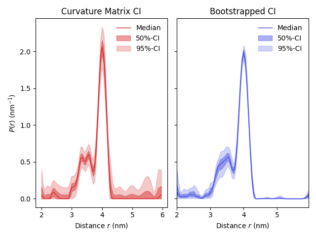
A simple example of uncertainty estimation of results obtained from dipolar signals. This example runs the analysis of a 4-pulse DEER signal and compares the uncertainty of the distance distribution between the moment-based (curvature matrix) and bootstrap methods.

By plotting the results, one can see that the bootstrapped confidence intervals are narrower in comparison to the ones obtained via the curvature matrices. This is because bootstrapping takes the nonnegativity constraint of P(r) into account, whereas the curvature matrix CIs do not.

import numpy as np
import matplotlib.pyplot as plt
import deerlab as dl

# File location
path = '../data/'
file = 'example_4pdeer_1.DTA'

# Experimental parameters
tau1 = 0.3      # First inter-pulse delay, μs
tau2 = 4.0      # Second inter-pulse delay, μs
tmin = 0.1      # Start time, μs

# Load the experimental data
t,Vexp = dl.deerload(path + file)

# Pre-processing
Vexp = dl.correctphase(Vexp) # Phase correction
Vexp = Vexp/np.max(Vexp)     # Rescaling (aesthetic)
t = t - t[0]                 # Account for zerotime
t = t + tmin

# Distance vector
r = np.arange(2,6,0.05) # nm

# Construct dipolar model
Vmodel = dl.dipolarmodel(t,r, experiment=dl.ex_4pdeer(tau1,tau2, pathways=[1]))

# Fit the model to the data using covariane-based uncertainty
results_cm = dl.fit(Vmodel,Vexp)

# Fit the model to the data using bootstrapped uncertainty
results_bs = dl.fit(Vmodel,Vexp,bootstrap=10)

# Compute the covariance-based uncertainty bands of the distance distribution
Pci50_cm = results_cm.PUncert.ci(50)
Pci95_cm = results_cm.PUncert.ci(95)

# Compute the bootstrapped uncertainty bands of the distance distribution
Pci50_bs = results_bs.PUncert.ci(50)
Pci95_bs = results_bs.PUncert.ci(95)

Bootstrap analysis with 1 cores:

  0%|          | 0/10 [00:00<?, ?it/s]
 10%|█         | 1/10 [00:03<00:30,  3.34s/it]
 20%|██        | 2/10 [00:05<00:20,  2.51s/it]
 30%|███       | 3/10 [00:07<00:17,  2.56s/it]
 40%|████      | 4/10 [00:11<00:16,  2.77s/it]
 50%|█████     | 5/10 [00:13<00:13,  2.69s/it]
 60%|██████    | 6/10 [00:17<00:11,  2.87s/it]
 70%|███████   | 7/10 [00:20<00:08,  2.89s/it]
 80%|████████  | 8/10 [00:23<00:05,  2.99s/it]
 90%|█████████ | 9/10 [00:27<00:03,  3.05s/it]
100%|██████████| 10/10 [00:31<00:00,  3.14s/it]
100%|██████████| 10/10 [00:31<00:00,  3.14s/it]
100%|██████████| 10/10 [00:31<00:00,  3.14s/it]

# Plot the results
fig, ax = plt.subplots(1,2,sharey=True)
violet = '#4550e6'

ax[0].plot(r,results_cm.P,'tab:red',linewidth=1)
ax[0].fill_between(r,Pci50_cm[:,0],Pci50_cm[:,1],color='tab:red',linestyle='None',alpha=0.45)
ax[0].fill_between(r,Pci95_cm[:,0],Pci95_cm[:,1],color='tab:red',linestyle='None',alpha=0.25)

ax[1].plot(r,results_bs.P,color=violet,linewidth=1)
ax[1].fill_between(r,Pci50_bs[:,0],Pci50_bs[:,1],color=violet,linestyle='None',alpha=0.45)
ax[1].fill_between(r,Pci95_bs[:,0],Pci95_bs[:,1],color=violet,linestyle='None',alpha=0.25)

ax[0].set_xlabel('Distance $r$ (nm)')
ax[0].set_ylabel('$P(r)$ (nm$^{-1}$)')
ax[0].set_title('Curvature Matrix CI')
ax[0].legend(['Median','50%-CI','95%-CI'],frameon=False,loc='best')

ax[1].set_xlabel('Distance $r$ (nm)')
ax[1].set_title('Bootstrapped CI')
ax[1].legend(['Median','50%-CI','95%-CI'],frameon=False,loc='best')

plt.autoscale(enable=True, axis='both', tight=True)
plt.tight_layout()
plt.show()