Bootstrapped confidence intervals in routine analysis

How to obtain bootstrapped confidence intervals for simple routine operations.

Unless specified otherwise, the function fit will return moment-based confidence intervals based on the covariance matrix of the objective function used to fit the data. These are quick to calculate and therefore very comfortable for quick estimates of the uncertainty during routine analysis or testing.

However, for publication-level analysis, these confidence intervals might be inaccurate. It is strongly recommended to employ bootstrapped confidence intervals to get accurate estimates of the uncertainty. Conviniently, fit integrates bootstrapping to make it accessible via the keyword argument bootstrap which specifies the number of samples to analyze to estimate the uncertainty. The larger this number, the more accurate the confidence intervals but the longer the analysis will be. The standard for publication is typically 1000 samples.

import numpy as np
import matplotlib.pyplot as plt
import deerlab as dl

# File location
path = '../data/'
file = 'example_4pdeer_1.DTA'

# Experimental parameters
tau1 = 0.3      # First inter-pulse delay, μs
tau2 = 4.0      # Second inter-pulse delay, μs
tmin = 0.1      # Start time, μs

# Load the experimental data
t,Vexp = dl.deerload(path + file)

# Pre-processing
Vexp = dl.correctphase(Vexp) # Phase correction
Vexp = Vexp/np.max(Vexp)     # Rescaling (aesthetic)
t = t - t[0]                 # Account for zerotime
t = t + tmin

# Distance vector
r = np.linspace(2,5,100) # nm

# Construct the model
Vmodel = dl.dipolarmodel(t,r, experiment = dl.ex_4pdeer(tau1,tau2, pathways=[1]))

# Fit the model to the data
results = dl.fit(Vmodel,Vexp,bootstrap=20)

# In this example, just for the sake of time, we will just use 20 bootstrap samples.

# Print results summary
print(results)

Bootstrap analysis with 1 cores:

  0%|          | 0/20 [00:00<?, ?it/s]
  5%|▌         | 1/20 [00:03<01:00,  3.17s/it]
 10%|█         | 2/20 [00:06<00:55,  3.07s/it]
 15%|█▌        | 3/20 [00:08<00:50,  2.96s/it]
 20%|██        | 4/20 [00:12<00:49,  3.08s/it]
 25%|██▌       | 5/20 [00:14<00:42,  2.85s/it]
 30%|███       | 6/20 [00:15<00:37,  2.66s/it]
 35%|███▌      | 7/20 [00:17<00:33,  2.55s/it]
 40%|████      | 8/20 [00:19<00:29,  2.47s/it]
 45%|████▌     | 9/20 [00:26<00:32,  2.91s/it]
 50%|█████     | 10/20 [00:29<00:29,  2.90s/it]
 55%|█████▌    | 11/20 [00:31<00:26,  2.90s/it]
 60%|██████    | 12/20 [00:36<00:24,  3.06s/it]
 65%|██████▌   | 13/20 [00:42<00:22,  3.24s/it]
 70%|███████   | 14/20 [00:49<00:21,  3.52s/it]
 75%|███████▌  | 15/20 [00:56<00:18,  3.75s/it]
 80%|████████  | 16/20 [01:03<00:15,  3.98s/it]
 85%|████████▌ | 17/20 [01:05<00:11,  3.84s/it]
 90%|█████████ | 18/20 [01:08<00:07,  3.79s/it]
 95%|█████████▌| 19/20 [01:11<00:03,  3.75s/it]
100%|██████████| 20/20 [01:14<00:00,  3.71s/it]
100%|██████████| 20/20 [01:14<00:00,  3.71s/it]
100%|██████████| 20/20 [01:14<00:00,  3.71s/it]
Goodness-of-fit:
========= ============= ============= ===================== =======
 Dataset   Noise level   Reduced 𝛘2    Residual autocorr.    RMSD
========= ============= ============= ===================== =======
   #1         0.005         0.812             0.124          0.004
========= ============= ============= ===================== =======
Model hyperparameters:
==========================
 Regularization parameter
==========================
          0.053
==========================
Model parameters:
=========== ========= ========================= ====== ======================================
 Parameter   Value     95%-Confidence interval   Unit   Description
=========== ========= ========================= ====== ======================================
 mod         0.303     (0.299,0.306)                    Modulation depth
 reftime     0.300     (0.298,0.302)              μs    Refocusing time
 conc        147.578   (143.904,151.590)          μM    Spin concentration
 P           ...       (...,...)                 nm⁻¹   Non-parametric distance distribution
 P_scale     1.004     (0.989,1.044)             None   Normalization factor of P
=========== ========= ========================= ====== ======================================

# Extract fitted dipolar signal
Vfit = results.model
Vci = results.propagate(Vmodel).ci(95)

# Extract fitted distance distribution
Pfit = results.P
Pci95 = results.PUncert.ci(95)
Pci50 = results.PUncert.ci(50)

# Extract the unmodulated contribution
Bfcn = lambda mod,conc,reftime: results.P_scale*(1-mod)*dl.bg_hom3d(t-reftime,conc,mod)
Bfit = results.evaluate(Bfcn)
Bci = results.propagate(Bfcn).ci(95)

plt.figure(figsize=[6,7])
violet = '#4550e6'
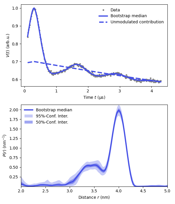
plt.subplot(211)
# Plot experimental data
plt.plot(t,Vexp,'.',color='grey',label='Data')
# Plot the fitted signal
plt.plot(t,Vfit,linewidth=3,label='Bootstrap median',color=violet)
plt.plot(t,Bfit,'--',linewidth=3,color=violet,label='Unmodulated contribution')
plt.legend(frameon=False,loc='best')
plt.xlabel('Time $t$ (μs)')
plt.ylabel('$V(t)$ (arb.u.)')
# Plot the distance distribution
plt.subplot(212)
plt.plot(r,Pfit,linewidth=3,label='Bootstrap median',color=violet)
plt.fill_between(r,Pci95[:,0],Pci95[:,1],alpha=0.3,color=violet,label='95%-Conf. Inter.',linewidth=0)
plt.fill_between(r,Pci50[:,0],Pci50[:,1],alpha=0.5,color=violet,label='50%-Conf. Inter.',linewidth=0)
plt.legend(frameon=False,loc='best')
plt.autoscale(enable=True, axis='both', tight=True)
plt.xlabel('Distance $r$ (nm)')
plt.ylabel('$P(r)$ (nm$^{-1}$)')
plt.tight_layout()
plt.show()