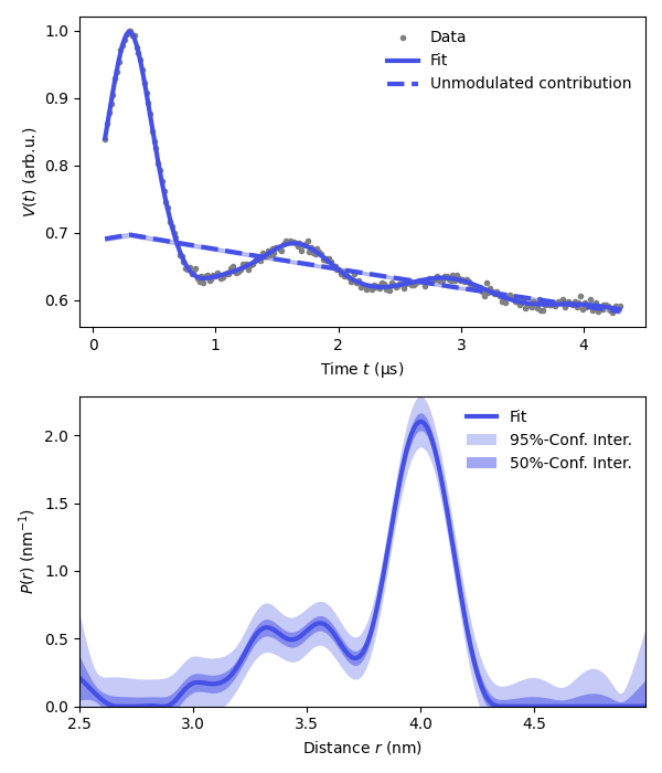
Basic analysis of a 4-pulse DEER signal

Fit a simple 4-pulse DEER signal with a model with a non-parametric distribution and a homogeneous background, using Tikhonov regularization.

import numpy as np
import matplotlib.pyplot as plt
import deerlab as dl

# File location
path = '../data/'
file = 'example_4pdeer_1.DTA'

# Experimental parameters
tau1 = 0.3      # First inter-pulse delay, μs
tau2 = 4.0      # Second inter-pulse delay, μs
tmin = 0.1      # Start time, μs

# Load the experimental data
t,Vexp = dl.deerload(path + file)

# Pre-processing
Vexp = dl.correctphase(Vexp) # Phase correction
Vexp = Vexp/np.max(Vexp)     # Rescaling (aesthetic)
t = t - t[0]                  # Account for zerotime
t = t + tmin
# Distance vector
r = np.arange(2.5,5,0.01) # nm

# Construct the model
Vmodel = dl.dipolarmodel(t,r, experiment = dl.ex_4pdeer(tau1,tau2, pathways=[1]))

# Fit the model to the data
results = dl.fit(Vmodel,Vexp)

# Print results summary
print(results)

Goodness-of-fit:
========= ============= ============= ===================== =======
 Dataset   Noise level   Reduced 𝛘2    Residual autocorr.    RMSD
========= ============= ============= ===================== =======
   #1         0.005         0.811             0.127          0.004
========= ============= ============= ===================== =======
Model hyperparameters:
==========================
 Regularization parameter
==========================
          0.224
==========================
Model parameters:
=========== ========= ========================= ====== ======================================
 Parameter   Value     95%-Confidence interval   Unit   Description
=========== ========= ========================= ====== ======================================
 mod         0.302     (0.299,0.305)                    Modulation depth
 reftime     0.299     (0.298,0.301)              μs    Refocusing time
 conc        148.470   (143.517,153.423)          μM    Spin concentration
 P           ...       (...,...)                 nm⁻¹   Non-parametric distance distribution
 P_scale     0.999     (0.998,1.000)             None   Normalization factor of P
=========== ========= ========================= ====== ======================================

# Extract fitted dipolar signal
Vfit = results.model

# Extract fitted distance distribution
Pfit = results.P
Pci95 = results.PUncert.ci(95)
Pci50 = results.PUncert.ci(50)

# Extract the unmodulated contribution
Bfcn = lambda mod,conc,reftime: results.P_scale*(1-mod)*dl.bg_hom3d(t-reftime,conc,mod)
Bfit = results.evaluate(Bfcn)
Bci = results.propagate(Bfcn).ci(95)

plt.figure(figsize=[6,7])
violet = '#4550e6'
plt.subplot(211)
# Plot experimental and fitted data
plt.plot(t,Vexp,'.',color='grey',label='Data')
plt.plot(t,Vfit,linewidth=3,color=violet,label='Fit')
plt.plot(t,Bfit,'--',linewidth=3,color=violet,label='Unmodulated contribution')
plt.fill_between(t,Bci[:,0],Bci[:,1],color=violet,alpha=0.3)
plt.legend(frameon=False,loc='best')
plt.xlabel('Time $t$ (μs)')
plt.ylabel('$V(t)$ (arb.u.)')
# Plot the distance distribution
plt.subplot(212)
plt.plot(r,Pfit,color=violet,linewidth=3,label='Fit')
plt.fill_between(r,Pci95[:,0],Pci95[:,1],alpha=0.3,color=violet,label='95%-Conf. Inter.',linewidth=0)
plt.fill_between(r,Pci50[:,0],Pci50[:,1],alpha=0.5,color=violet,label='50%-Conf. Inter.',linewidth=0)
plt.legend(frameon=False,loc='best')
plt.autoscale(enable=True, axis='both', tight=True)
plt.xlabel('Distance $r$ (nm)')
plt.ylabel('$P(r)$ (nm$^{-1}$)')
plt.tight_layout()
plt.show()