Note
Go to the end to download the full example code.
Global analysis of 5-pulse DEER on a liquid-droplet protein system
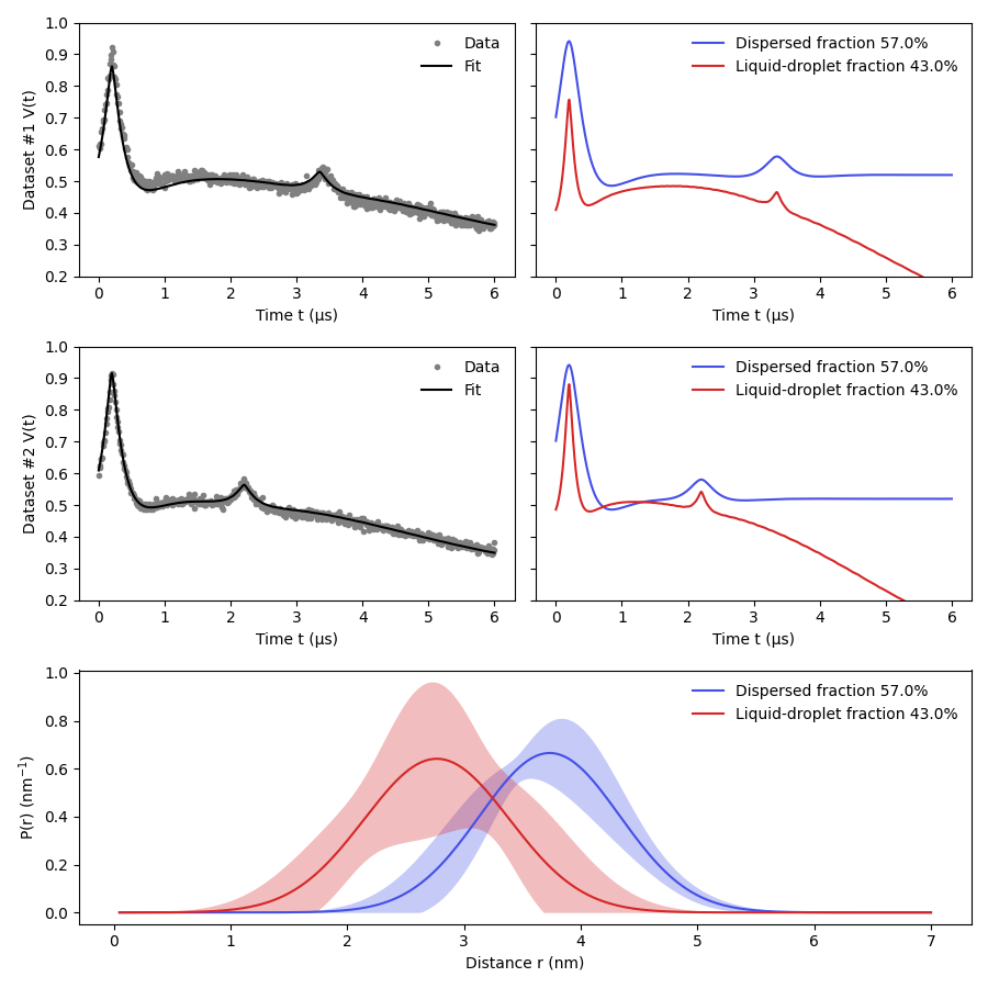
Certain protein systems can form fractions of protein either in a liquid-droplet or dispersed states. Each of these fractions gives rise to a different dipolar signal which are combined into a detected signal. Due to the differences in local concentration the intermolecular contributions for each fraction are completely different and can be modelled in a global manner.
As in the publication referenced below, this example will take two 5-pulse DEER signals acquired on the same sample with slightly different pulse sequence delays and fit it globally to the droplet signal model.
For the original model and more information on these systems please refer to: Emmanouilidis, L., Esteban-Hofer, L., Damberger, F.F. et al. NMR and EPR reveal a compaction of the RNA-binding protein FUS upon droplet formation. Nat Chem Biol 17, 608–614 (2021). https://doi.org/10.1038/s41589-021-00752-3
Goodness-of-fit:
========= ============= ============= ===================== =======
 Dataset   Noise level   Reduced 𝛘2    Residual autocorr.    RMSD
========= ============= ============= ===================== =======
   #1         0.011         2.480             1.271          0.017
   #2         0.008         1.554             0.582          0.009
========= ============= ============= ===================== =======
Model hyperparameters:
==========================
 Regularization parameter
==========================
         0.00e+00
==========================
Model parameters:
============ ========== ========================= ====== ===============================
 Parameter    Value      95%-Confidence interval   Unit   Description
============ ========== ========================= ====== ===============================
 lam1         0.422      (0.411,0.433)                    Amplitude of pathway #1
 reftime1     0.198      (0.196,0.201)              μs    Refocusing time of pathway #1
 lam2         0.059      (0.053,0.064)                    Amplitude of pathway #2
 reftime2_1   3.351      (3.328,3.375)              μs    Refocusing time of pathway #2
 kdis         8.39e-22   (0.00e+00,0.018)          μs⁻¹   Decay rate
 rmean_dis    3.735      (3.546,3.923)              nm    Mean
 std_dis      0.599      (0.481,0.718)              nm    Standard deviation
 eta          0.570      (0.468,0.570)             None   Weighting factor
 kld          0.011      (0.005,0.016)             μs⁻¹   Decay rate
 Dld          2.635      (2.144,3.127)                    Stretch factor
 rmean_ld     2.768      (2.486,3.049)              nm    Mean
 std_ld       0.622      (0.313,0.931)              nm    Standard deviation
 reftime2_2   2.205      (2.195,2.215)              μs    Refocusing time of pathway #2
 scale_1_1    1.000      (frozen)                  None   Overall echo amplitude/scale
 scale_2_1    1.000      (frozen)                  None   Overall echo amplitude/scale
 scale_1_2    1.000      (frozen)                  None   Overall echo amplitude/scale
 scale_2_2    1.000      (frozen)                  None   Overall echo amplitude/scale
============ ========== ========================= ====== ===============================
import deerlab as dl
import numpy as np
import matplotlib.pyplot as plt
violet = '#4550e6'


# Load experimental data
t1,Vexp1 = np.load('../data/example_droplets_data_1.npy')
t2,Vexp2 = np.load('../data/example_droplets_data_2.npy')

# Put all datasets into lists
ts = [t1,t2]
Vs = [Vexp1,Vexp2]

# Distance vector
r = np.linspace(0.05,7,200)

# Model of a dipolar signal in arising from a dispersed and liquid-droplet states
#----------------------------------------------------------------------------------
def dropletmodel(t):
    # Dispersed-state component model
    Vdis_model = dl.dipolarmodel(t,r, Pmodel=dl.dd_gauss, Bmodel=dl.bg_exp, npathways=2)
    # Liquid-droplet-state component model
    Vld_model = dl.dipolarmodel(t,r, Pmodel=dl.dd_gauss, Bmodel=dl.bg_strexp, npathways=2)
    # Create a dipolar signal model that is a linear combination of both components
    Vmodel = dl.lincombine(Vdis_model,Vld_model, addweights=True)
    Vmodel = dl.link(Vmodel,
                    reftime1=['reftime1_1','reftime1_2'],
                    reftime2=['reftime2_1','reftime2_2'],
                    lam1=['lam1_1','lam1_2'],
                    lam2=['lam2_1','lam2_2'])
    Vmodel.scale_1.freeze(1)
    Vmodel.scale_2.freeze(1)
    # Make the second weight dependent on the first one
    Vmodel = dl.relate(Vmodel,weight_2 = lambda weight_1: 1 - weight_1)
    return Vmodel,Vdis_model,Vld_model
#----------------------------------------------------------------------------------

# Generate the models
Vmodel1,Vdismodel1,Vldmodel1 = dropletmodel(ts[0])
Vmodel2,Vdismodel2,Vldmodel2 = dropletmodel(ts[1])

# Create the global model
globalModel = dl.merge(Vmodel1,Vmodel2)
# Link global parameters toghether with new names
globalModel = dl.link(globalModel,
                eta = ['weight_1_1','weight_1_2'],
                kdis = ['decay_1_1','decay_1_2'],
                kld = ['decay_2_1','decay_2_2'],
                Dld = ['stretch_2_1','stretch_2_2'],
                rmean_dis = ['mean_1_1','mean_1_2'],
                rmean_ld = ['mean_2_1','mean_2_2'],
                std_dis = ['std_1_1','std_1_2'],
                std_ld = ['std_2_1','std_2_2'],
                lam1 = ['lam1_1','lam1_2'],
                lam2 = ['lam2_1','lam2_2'],
                reftime1 = ['reftime1_1','reftime1_2'])

# Specify parameter boundaries and initial conditions
globalModel.eta.set(       lb=0.468, ub=0.57, par0=0.520)
globalModel.kdis.set(      lb=0.0,   ub=0.09, par0=0.01)
globalModel.kld.set(       lb=0.0,   ub=1,    par0=0.12)
globalModel.Dld.set(       lb=2,     ub=4,    par0=2.5)
globalModel.rmean_dis.set( lb=3,     ub=6.35, par0=3.7)
globalModel.rmean_ld.set(  lb=1,     ub=4.35, par0=2.6)
globalModel.std_dis.set(   lb=0.25,  ub=0.74, par0=0.44)
globalModel.std_ld.set(    lb=0.2,   ub=2,    par0=0.7)
globalModel.lam1.set(      lb=0.3,   ub=0.5,  par0=0.4)
globalModel.lam2.set(      lb=0.0,   ub=0.2,  par0=0.08)
globalModel.reftime1.set(  lb=0.1,   ub=0.3,  par0=0.2)
globalModel.reftime2_1.set(lb=3.2,   ub=3.8,  par0=3.4)
globalModel.reftime2_2.set(lb=2.0,   ub=2.5,  par0=2.2)

# Fit the model to the data
fit = dl.fit(globalModel,Vs)

print(fit)

# Plot the results
plt.figure(figsize=[9,9])
violet = '#4550e6'

plt.subplot(3,2,1)
plt.plot(ts[0],Vs[0],'.',color='grey',label='Data')
plt.plot(ts[0],fit.model[0],color='k',label='Fit',linewidth=1.5)
plt.ylim([0.2,1])
plt.legend(frameon=False,loc='best')
plt.xlabel('Time t (μs)')
plt.ylabel('Dataset #1 V(t)')

ax2 = plt.subplot(3,2,2)

Vdis_fit = Vdismodel1(decay=fit.kdis,mean=fit.rmean_dis,std=fit.std_dis,reftime1=fit.reftime1,reftime2=fit.reftime2_1,lam1=fit.lam1,lam2=fit.lam2,scale=1)
Vld_fit = Vldmodel1(decay=fit.kld,stretch=fit.Dld,mean=fit.rmean_ld,std=fit.std_ld,reftime1=fit.reftime1,reftime2=fit.reftime2_1,lam1=fit.lam1,lam2=fit.lam2,scale=1)

ax2.plot(ts[0],Vdis_fit,color=violet,label=f'Dispersed fraction {fit.eta*100:.1f}%')
ax2.plot(ts[0],Vld_fit,color='tab:red',label=f'Liquid-droplet fraction {(1-fit.eta)*100:.1f}%')
ax2.set_yticklabels([])
ax2.legend(frameon=False,loc='best')
ax2.set_ylim([0.2,1])
ax2.set_xlabel('Time t (μs)')


plt.subplot(3,2,3)
plt.plot(ts[1],Vs[1],'.',color='grey',label='Data')
plt.plot(ts[1],fit.model[1],color='k',label='Fit',linewidth=1.5)
plt.ylim([0.2,1])
plt.legend(frameon=False,loc='best')
plt.xlabel('Time t (μs)')
plt.ylabel('Dataset #2 V(t)')

ax4 = plt.subplot(3,2,4)

Vdis_fit = Vdismodel2(decay=fit.kdis,mean=fit.rmean_dis,std=fit.std_dis,reftime1=fit.reftime1,reftime2=fit.reftime2_2,lam1=fit.lam1,lam2=fit.lam2,scale=1)
Vld_fit = Vldmodel2(decay=fit.kld,stretch=fit.Dld,mean=fit.rmean_ld,std=fit.std_ld,reftime1=fit.reftime1,reftime2=fit.reftime2_2,lam1=fit.lam1,lam2=fit.lam2,scale=1)

ax4.plot(ts[1],Vdis_fit,color=violet,label=f'Dispersed fraction {fit.eta*100:.1f}%')
ax4.plot(ts[1],Vld_fit,color='tab:red',label=f'Liquid-droplet fraction {(1-fit.eta)*100:.1f}%')
ax4.set_yticklabels([])
ax4.legend(frameon=False,loc='best')
ax4.set_xlabel('Time t (μs)')
ax4.set_ylim([0.2,1])

plt.subplot(3,1,3)

Pdis_fcn = lambda rmean_dis,std_dis: dl.dd_gauss(r,rmean_dis,std_dis)
Pld_fcn = lambda rmean_ld,std_ld: dl.dd_gauss(r,rmean_ld,std_ld)

Pdis_uq = fit.propagate(Pdis_fcn,lb=np.zeros_like(r))
Pld_uq = fit.propagate(Pld_fcn,lb=np.zeros_like(r))

plt.plot(r,Pdis_fcn(fit.rmean_dis,fit.std_dis),label=f'Dispersed fraction {fit.eta*100:.1f}%',color=violet)
plt.fill_between(r,Pdis_uq.ci(95)[:,0],Pdis_uq.ci(95)[:,1],alpha=0.3,linewidth=0,color=violet)
plt.plot(r,Pld_fcn(fit.rmean_ld,fit.std_ld),label=f'Liquid-droplet fraction {(1-fit.eta)*100:.1f}%',color='tab:red')
plt.fill_between(r,Pld_uq.ci(95)[:,0],Pld_uq.ci(95)[:,1],alpha=0.3,linewidth=0,color='tab:red')

plt.legend(frameon=False,loc='best')
plt.xlabel('Distance r (nm)')
plt.ylabel('P(r) (nm$^{-1}$)')
plt.tight_layout()
plt.show()
Total running time of the script: (0 minutes 30.484 seconds)