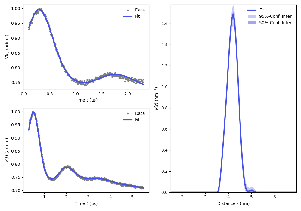
Global fitting of multiple 4-pulse DEER signals, non-parametric distribution

How to fit multiple 4-pulse DEER signals to a model with a non-parametric distribution and a homogeneous background.

import numpy as np
import matplotlib.pyplot as plt
import deerlab as dl

# File location
path = '../data/'
files = [
    'example_4pdeer_3.DTA',
    'example_4pdeer_4.DTA',
    ]

# Experimental parameters
tau1s = [0.3, 0.5]      # First inter-pulse delay, μs
tau2s = [2.0, 4.0]      # Second inter-pulse delay, μs
tmins = [0.1, 0.3]      # Start time, μs

Vmodels,ts,Vs = [],[],[]
for file, tau1, tau2, tmin in zip(files, tau1s, tau2s, tmins):

    # Load the experimental data
    t,Vexp = dl.deerload(path + file)

    # Pre-processing
    Vexp = dl.correctphase(Vexp) # Phase correction
    Vexp = Vexp/np.max(Vexp)     # Rescaling (aesthetic)
    t = t - t[0]                     # Account for zerotime
    t = t + tmin

    # Distance vector
    r = np.arange(1.5,7,0.05) # nm

    # Put the datasets into lists
    ts.append(t)
    Vs.append(Vexp)

    # Construct the dipolar models for the individual signals
    Vmodels.append(dl.dipolarmodel(t,r, experiment=dl.ex_4pdeer(tau1,tau2,pathways=[1])) )

# Make the global model by joining the individual models
globalmodel = dl.merge(*Vmodels)

# Link the distance distribution into a global parameter
globalmodel = dl.link(globalmodel,P=['P_1','P_2'])

# Compactness criterion for the global distance distribution
compactness = dl.dipolarpenalty(Pmodel=None,r=r,type='compactness')

# Fit the model to the data
results = dl.fit(globalmodel,Vs, weights=[1,1],penalties=compactness)

plt.figure(figsize=[10,7])
violet = '#4550e6'
for n in range(len(results.model)):

    # Extract fitted dipolar signal
    Vfit = results.model[n]

    # Extract fitted distance distribution
    Pfit = results.P
    Pci95 = results.PUncert.ci(95)
    Pci50 = results.PUncert.ci(50)

    plt.subplot(2,2,2*n+1)
    # Plot experimental data
    plt.plot(ts[n],Vs[n],'.',color='grey',label='Data')
    # Plot the fitted signal
    plt.plot(ts[n],Vfit,linewidth=3,color=violet,label='Fit')
    plt.legend(frameon=False,loc='best')
    plt.xlabel('Time $t$ (μs)')
    plt.ylabel('$V(t)$ (arb.u.)')

# Plot the distance distribution
plt.subplot(122)
plt.plot(r,Pfit,linewidth=3,label='Fit',color=violet)
plt.fill_between(r,Pci95[:,0],Pci95[:,1],alpha=0.3,color=violet,label='95%-Conf. Inter.',linewidth=0)
plt.fill_between(r,Pci50[:,0],Pci50[:,1],alpha=0.5,color=violet,label='50%-Conf. Inter.',linewidth=0)
plt.legend(frameon=False,loc='best')
plt.autoscale(enable=True, axis='both', tight=True)
plt.xlabel('Distance $r$ (nm)')
plt.ylabel('$P(r)$ (nm$^{-1}$)')
plt.tight_layout()
plt.show()