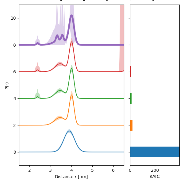
Multi-Gaussian analysis of a dipolar signal

An example on how to perform a multi-Gauss analysis of dipolar signals using optimal selection of the number of components.

# Import the required libraries
import numpy as np
import matplotlib.pyplot as plt
from matplotlib.gridspec import GridSpec
from copy import deepcopy
import deerlab as dl

# File location
path = "../data/"
file = "example_4pdeer_1.DTA"

# Experimental parameters
tau1 = 0.3  # First inter-pulse delay, μs
tau2 = 4.0  # Second inter-pulse delay, μs
tmin = 0.1  # Start time, μs

# Load the experimental data
t, Vexp = dl.deerload(path + file)

# Pre-processing
Vexp = dl.correctphase(Vexp)    # Phase correction
Vexp = Vexp / np.max(Vexp)      # Rescaling (aesthetic)
t = t - t[0]                    # Account for zerotime
t = t + tmin

# Maximal number of Gaussians in the models
Nmax = 5

# Construct the distance axis
r = np.linspace(1.5, 6.5, 500)

# Pre-allocate the empty lists of models
Pmodels = [[] for _ in range(Nmax)]
Vmodels = [[] for _ in range(Nmax)]

# The basic model for the components (can be e.g. dl.dd_rice)
basisModel = deepcopy(dl.dd_gauss)
basisModel.mean.set(lb=min(r), ub=max(r), par0=3.5)

# Model construction
for n in range(Nmax):
    # Construct the n-Gaussian model
    Pmodels[n] = dl.lincombine(*[basisModel] * (n + 1))
    # Construct the corresponding dipolar signal model
    Vmodels[n] = dl.dipolarmodel(t, r, Pmodel=Pmodels[n])

# Fit the models to the data
fits = [[] for _ in range(Nmax)]
for n in range(Nmax):
    fits[n] = dl.fit(Vmodels[n], Vexp, reg=False)

# Extract the values of the Akaike information criterion for each fit
aic = np.array([fit.stats["aic"] for fit in fits])
# Compute the relative difference in AIC
aic -= aic.min()

# Plotting
fig = plt.figure(figsize=[6, 6])
gs = GridSpec(1, 3, figure=fig)
ax1 = fig.add_subplot(gs[0, :-1])
for n in range(Nmax):
    # Evaluate the n-Gaussian distance distribution model
    Pfit = fits[n].evaluate(Pmodels[n], *[r] * (n + 1))
    # Propagate the fit uncertainty to the model
    Puq = fits[n].propagate(Pmodels[n], *[r] * (n + 1), lb=np.zeros_like(r))
    # Calculate the 95%-confidence intervals
    Pci = Puq.ci(95)
    # Normalize the probability density functions
    Pci /= np.trapz(Pfit, r)
    Pfit /= np.trapz(Pfit, r)
    # Plot the optimal fit with a thicker line
    if n == np.argmin(aic):
        lw = 4
    else:
        lw = 1.5
    # Plot the distance distributions and their confidence bands
    ax1.plot(r, n * 2 + Pfit, label=f"{1+n}", linewidth=lw)
    ax1.fill_between(r, n * 2 + Pci[:, 0], n * 2 + Pci[:, 1], alpha=0.3)

# Plot the difference in AIC for each fit
ax2 = fig.add_subplot(gs[0, -1])
for n in range(Nmax):
    ax2.barh(2 * n, aic[n])

# Axes settings
ax1.set_ylabel("P(r)")
ax1.set_xlabel("Distance $r$ [nm]")
ax1.set_ylim([-1, 2 * Nmax + 1])
ax1.autoscale(enable=True, axis="x", tight=True)
ax2.set_xlabel("$\Delta$AIC")
ax2.set_ylim([-1, 2 * Nmax + 1])
ax2.autoscale(enable=True, axis="x", tight=True)
ax2.yaxis.set_ticklabels([])
# Legend settings
handles, labels = ax1.get_legend_handles_labels()
fig.legend(
    handles,
    labels,
    title="N-Gaussian model",
    frameon=False,
    loc="upper center",
    ncol=Nmax,
    bbox_to_anchor=(0.55, 1.07),
)
plt.tight_layout()
plt.show()