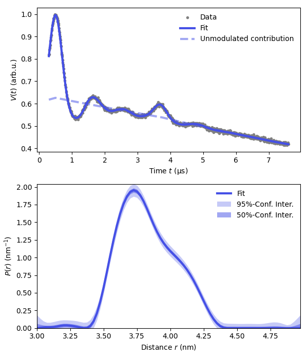
Basic fitting of a 5-pulse DEER signal

This example shows how to model and fit a 5-pulse DEER signal, including the typically present additional dipolar pathway.

Now, the simple 5pDEER models contain 3 additional parameters compared to 4pDEER (due to the additional dipolar pathway present in the signal). However, the refocusing time of the second dipolar pathway is very easy to constrain and strongly helps stabilizing the results.

This pathway can even estimated visually from the signal or estimated from the pulse sequence timings. Thus, we can strongly constraint this parameters while leaving the pathway amplitudes pretty much unconstrained.

Import required packages

import numpy as np
import matplotlib.pyplot as plt
import deerlab as dl

# File location
path = '../data/'
file = 'example_5pdeer_1.DTA'

# Experimental parameters (reversed 5pDEER)
tau1 = 3.9              # First inter-pulse delay, μs
tau2 = 3.7              # Second inter-pulse delay, μs
tau3 = 0.5              # Third inter-pulse delay, μs
tmin = 0.3              # Start time, μs

# Load the experimental data
t,Vexp = dl.deerload(path + file)
Vexp = dl.correctphase(Vexp)    # Phase correction
Vexp = Vexp/np.max(Vexp)        # Rescaling (aesthetic)
t = t - t[0]                    # Account for zerotime
t = t + tmin

# Distance vector
r = np.arange(3,5,0.025) # nm

# Construct dipolar model with two dipolar pathways
experimentInfo = dl.ex_rev5pdeer(tau1, tau2, tau3, pathways=[1,5])
Vmodel = dl.dipolarmodel(t,r, experiment=experimentInfo)

# Fit the model to the data
results = dl.fit(Vmodel,Vexp)

# Print results summary
print(results)

Goodness-of-fit:
========= ============= ============= ===================== =======
 Dataset   Noise level   Reduced 𝛘2    Residual autocorr.    RMSD
========= ============= ============= ===================== =======
   #1         0.004         0.979             0.082          0.004
========= ============= ============= ===================== =======
Model hyperparameters:
==========================
 Regularization parameter
==========================
          0.104
==========================
Model parameters:
=========== ========= ========================= ====== ======================================
 Parameter   Value     95%-Confidence interval   Unit   Description
=========== ========= ========================= ====== ======================================
 lam1        0.349     (0.348,0.351)                    Amplitude of pathway #1
 reftime1    0.500     (0.499,0.502)              μs    Refocusing time of pathway #1
 lam5        0.061     (0.059,0.062)                    Amplitude of pathway #5
 reftime5    3.701     (3.691,3.710)              μs    Refocusing time of pathway #5
 conc        160.372   (159.220,161.525)          μM    Spin concentration
 P           ...       (...,...)                 nm⁻¹   Non-parametric distance distribution
 P_scale     1.095     (1.094,1.095)             None   Normalization factor of P
=========== ========= ========================= ====== ======================================

# Extract fitted dipolar signal
Vfit = results.model
Vci = results.propagate(Vmodel).ci(95)

# Extract fitted distance distribution
Pfit = results.P
Pci95 = results.PUncert.ci(95)
Pci50 = results.PUncert.ci(50)
Pfit =  Pfit

# Extract the unmodulated contribution
Bfcn = lambda lam1,lam5,reftime1,reftime5,conc: results.P_scale*(1-lam1-lam5)*dl.bg_hom3d(t-reftime1,conc,lam1)*dl.bg_hom3d(t-reftime5,conc,lam5)
Bfit = results.evaluate(Bfcn)
Bci = results.propagate(Bfcn).ci(95)

plt.figure(figsize=[6,7])
violet = '#4550e6'
plt.subplot(211)
# Plot experimental data
plt.plot(t,Vexp,'.',color='grey',label='Data')
# Plot the fitted signal
plt.plot(t,Vfit,linewidth=3,color=violet,label='Fit')
plt.plot(t,Bfit,'--',linewidth=3,color=violet,alpha=0.5,label='Unmodulated contribution')
plt.legend(frameon=False,loc='best')
plt.xlabel('Time $t$ (μs)')
plt.ylabel('$V(t)$ (arb.u.)')
# Plot the distance distribution
plt.subplot(212)
plt.plot(r,Pfit,linewidth=3,color=violet,label='Fit')
plt.fill_between(r,Pci95[:,0],Pci95[:,1],alpha=0.3,color=violet,label='95%-Conf. Inter.',linewidth=0)
plt.fill_between(r,Pci50[:,0],Pci50[:,1],alpha=0.5,color=violet,label='50%-Conf. Inter.',linewidth=0)
plt.legend(frameon=False,loc='best')
plt.autoscale(enable=True, axis='both', tight=True)
plt.xlabel('Distance $r$ (nm)')
plt.ylabel('$P(r)$ (nm$^{-1}$)')
plt.tight_layout()
plt.show()