Distance restraints from 4-pulse DEER data, non-parametric distribution

How to fit a simple 4-pulse DEER signal and derive distance restraints from the fitted non-parametric distance distribution.

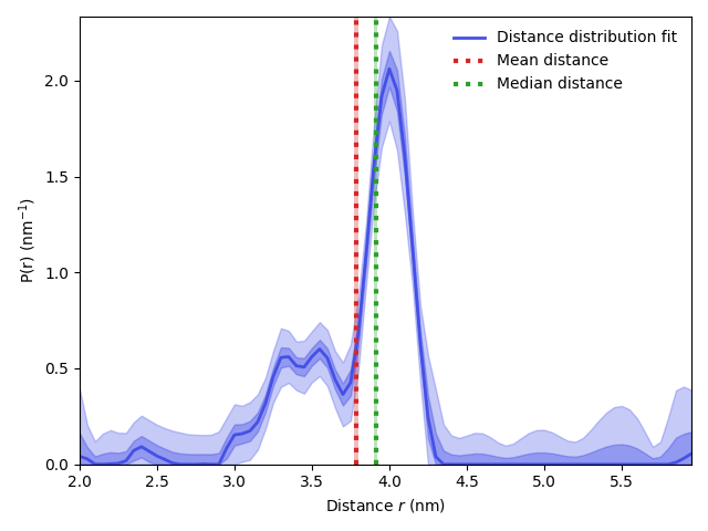
Once we have a fit of the distance distribution we can obtain distance restraints in the form of different statistical descriptors such as the mean distance and standard deviation of distances. While we could calculate this manually, DeerLab provides a convenient function diststats which will automatically compute these for you and even propagate the uncertainty in the distributions to those values to get confidence intervals on the restraints.

import numpy as np
import matplotlib.pyplot as plt
import deerlab as dl

# File location
path = '../data/'
file = 'example_4pdeer_1.DTA'

# Experimental parameters
tau1 = 0.3      # First inter-pulse delay, μs
tau2 = 4.0      # Second inter-pulse delay, μs
tmin = 0.1      # Start time, μs

# Load the experimental data
t,Vexp = dl.deerload(path + file)

# Pre-processing
Vexp = dl.correctphase(Vexp) # Phase correction
Vexp = Vexp/np.max(Vexp)     # Rescaling (aesthetic)
t = t + tmin                # Account for zerotime

# Distance vector
r = np.arange(2,6,0.05) # nm

# Construct dipolar model
Vmodel = dl.dipolarmodel(t,r, experiment=dl.ex_4pdeer(tau1,tau2, pathways=[1]))

# Fit the model to the data
fit = dl.fit(Vmodel,Vexp)

# Get printed summary of all statistical descriptors available with confidence intervals
estimators,uq = dl.diststats(r,fit.P,fit.PUncert,verbose=True)

# Get the mean distance
rmean = estimators['mean']
rmean_ci = uq['mean'].ci(95)
# Get the median distance
rmedian = estimators['median']
rmedian_ci = uq['median'].ci(95)
# Get the standard deviation of distances
r_std = estimators['std']
r_std_ci = uq['std'].ci(95)

# Print out the results
print(f'Mean distance: {rmean:.3f} ({rmean_ci[0]:.3f}-{rmean_ci[1]:.3f}) nm')
print(f'Standard deviation: {r_std:.3f} ({r_std_ci[0]:.3f}-{r_std_ci[1]:.3f}) nm')

-------------------------------------------------
Distribution Statistics
-------------------------------------------------
Range                    2.00-5.95 nm
Integral                 1.00
-------------------------------------------------
Location
-------------------------------------------------
Range                    2.00-5.95 nm
Mean                     3.79 (3.77,3.80) nm
Median                   3.91 (3.90,3.92) nm
Interquartile mean       3.87 (3.86,3.88) nm
Mode                     4.00 nm
-------------------------------------------------
Spread
-------------------------------------------------
Standard deviation       0.39 (0.32,0.46) nm
Mean absolute deviation  0.30 (0.28,0.31) nm
Interquartile range      0.49 (0.46,0.51) nm
Variance                 0.15 (0.10,0.20) nm²
-------------------------------------------------
Shape
-------------------------------------------------
Modality                 3
Skewness                 -0.74 (-3.46,1.97)
Kurtosis                 -4.80 (-19.37,9.78)
-------------------------------------------------
Mean distance: 3.788 (3.773-3.803) nm
Standard deviation: 0.388 (0.319-0.456) nm

# For display, you can plot the mean distance with its confidence intervals without further calculations.

# Plot distribution and confidence bands
violet = '#4550e6'
Pci95 = fit.PUncert.ci(95)/np.trapz(fit.P,r)
Pci50 = fit.PUncert.ci(50)/np.trapz(fit.P,r)
plt.plot(r,fit.P/np.trapz(fit.P,r),linewidth=2,color=violet,label='Distance distribution fit')
plt.fill_between(r,Pci95[:,0],Pci95[:,1],color=violet,alpha=0.3)
plt.fill_between(r,Pci50[:,0],Pci50[:,1],color=violet,alpha=0.4)

# Plot mean distance and confidence interval
plt.vlines(rmean,0,max(Pci95[:,1]),color='tab:red',linestyles='dotted',linewidth=3,label='Mean distance')
plt.vlines(rmedian,0,max(Pci95[:,1]),color='tab:green',linestyles='dotted',linewidth=3,label='Median distance')
plt.fill_between(rmean_ci,0,max(Pci95[:,1]),color='tab:red',alpha=0.3,linewidth=0)
plt.fill_between(rmedian_ci,0,max(Pci95[:,1]),color='tab:green',alpha=0.3,linewidth=0)

plt.legend(frameon=False,loc='best')

plt.ylim([0,max(Pci95[:,1])])
plt.xlabel('Distance $r$ (nm)')
plt.ylabel('P(r) (nm$^{-1}$)')
plt.autoscale(enable=True, axis='both', tight=True)
plt.tight_layout()
plt.show()