Validating multi-pathway models based on the data

How to determine whether the dipolar signal model defined with the set of specified dipolar pathways pathways is a proper descriptor of the experimental data.

This example shows how to use goodness-of-fit criteria to determine whether enough dipolar pathways have been accounted for in the model.

A model that accurately describes the data must result in a residual vector that is normally distributed, has zero mean, and has no significant autocorrelations. In this example, we will look at an experimental 4-pulse DEER dataset acquired on a maltose-binding protein (MBP) and use the built-in goodness-of-fit tools to quantitatively validate whether the dataste is well described by a dipolar model with a single, two or three dipolar pathways.

import numpy as np
import deerlab as dl
import matplotlib.pyplot as plt

# File location
file = "../data/experimental_mbp_protein_4pdeer.DTA"

# Experiment information
tmin = 0.040
tau1 = 0.4
tau2 = 3.0

# Laod and preprocess the data
t,Vexp = dl.deerload(file)
t = t[:-2]
Vexp = Vexp[:-2]
Vexp = dl.correctphase(Vexp)
Vexp = Vexp/max(Vexp)
t = t- t[0] + tmin

# Define the distance vector
r = np.arange(3,4.5,0.05)

# Loop over different dipolar models with varying number of pathways
for Npathways in [1,2,3]:
    print(f'Model with {Npathways} dipolar pathways:')

    # Construct the experiment model with different pathways
    experiment = dl.ex_4pdeer(tau1,tau2,pathways=np.arange(1,Npathways+1,1))

    # Construct the dipolar model with a non-parametric distance distribution
    Vmodel = dl.dipolarmodel(t,r,experiment=experiment)

    # Define the compactness penalty for best results
    compactness = dl.dipolarpenalty(None,r,'compactness')

    # Fit the data to the current model
    results = dl.fit(Vmodel,Vexp,penalties=compactness)

    # Print the summary of the results
    print(results)

    # Plot the fit of the model to the data along its goodness-of-fit tests
    results.plot(axis=t, xlabel='t (μs)', gof=True)
    plt.suptitle(f'Model with {Npathways} dipolar pathways:')
    plt.show()

• 
• 
• 

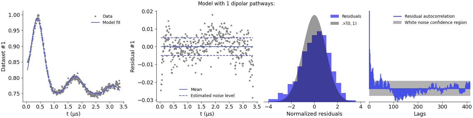
Model with 1 dipolar pathways:
Goodness-of-fit:
========= ============= ============= ===================== =======
 Dataset   Noise level   Reduced 𝛘2    Residual autocorr.    RMSD
========= ============= ============= ===================== =======
   #1         0.005         1.868             1.056          0.007
========= ============= ============= ===================== =======
Model hyperparameters:
========================== ===================
 Regularization parameter   Penalty weight #1
========================== ===================
          0.002                   0.059
========================== ===================
Model parameters:
=========== ========= ========================= ====== ======================================
 Parameter   Value     95%-Confidence interval   Unit   Description
=========== ========= ========================= ====== ======================================
 mod         0.189     (0.186,0.192)                    Modulation depth
 reftime     0.390     (0.387,0.394)              μs    Refocusing time
 conc        113.705   (105.902,121.508)          μM    Spin concentration
 P           ...       (...,...)                 nm⁻¹   Non-parametric distance distribution
 P_scale     0.989     (0.988,0.989)             None   Normalization factor of P
=========== ========= ========================= ====== ======================================

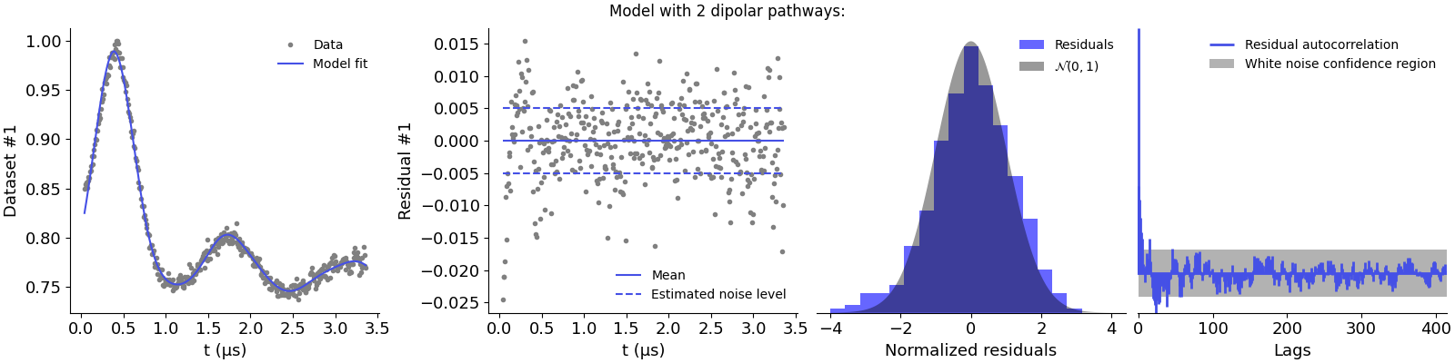
Model with 2 dipolar pathways:
Goodness-of-fit:
========= ============= ============= ===================== =======
 Dataset   Noise level   Reduced 𝛘2    Residual autocorr.    RMSD
========= ============= ============= ===================== =======
   #1         0.005         1.433             0.766          0.006
========= ============= ============= ===================== =======
Model hyperparameters:
========================== ===================
 Regularization parameter   Penalty weight #1
========================== ===================
          0.006                   0.008
========================== ===================
Model parameters:
=========== ========= ========================= ====== ======================================
 Parameter   Value     95%-Confidence interval   Unit   Description
=========== ========= ========================= ====== ======================================
 lam1        0.182     (0.179,0.184)                    Amplitude of pathway #1
 reftime1    0.385     (0.382,0.389)              μs    Refocusing time of pathway #1
 lam2        0.036     (0.031,0.042)                    Amplitude of pathway #2
 reftime2    3.352     (3.352,3.390)              μs    Refocusing time of pathway #2
 conc        173.512   (160.834,186.190)          μM    Spin concentration
 P           ...       (...,...)                 nm⁻¹   Non-parametric distance distribution
 P_scale     1.048     (1.047,1.049)             None   Normalization factor of P
=========== ========= ========================= ====== ======================================

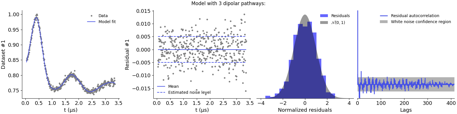
Model with 3 dipolar pathways:
Goodness-of-fit:
========= ============= ============= ===================== =======
 Dataset   Noise level   Reduced 𝛘2    Residual autocorr.    RMSD
========= ============= ============= ===================== =======
   #1         0.005         1.054             0.306          0.005
========= ============= ============= ===================== =======
Model hyperparameters:
========================== ===================
 Regularization parameter   Penalty weight #1
========================== ===================
          0.004                   0.046
========================== ===================
Model parameters:
=========== ========= ========================= ====== ======================================
 Parameter   Value     95%-Confidence interval   Unit   Description
=========== ========= ========================= ====== ======================================
 lam1        0.180     (0.175,0.184)                    Amplitude of pathway #1
 reftime1    0.414     (0.406,0.422)              μs    Refocusing time of pathway #1
 lam2        0.035     (0.029,0.041)                    Amplitude of pathway #2
 reftime2    3.358     (3.352,3.401)              μs    Refocusing time of pathway #2
 lam3        0.038     (0.032,0.045)                    Amplitude of pathway #3
 reftime3    -0.031    (-0.048,0.048)             μs    Refocusing time of pathway #3
 conc        128.848   (116.625,141.070)          μM    Spin concentration
 P           ...       (...,...)                 nm⁻¹   Non-parametric distance distribution
 P_scale     1.088     (1.088,1.089)             None   Normalization factor of P
=========== ========= ========================= ====== ======================================

The first model is clearly underparametrized as it results in non-normal residuals and strong correlations. This is supported by the large chi-squared value. Adding the second pathway seems to improve the description of the data, as the residuals are now better distributed. However, there appears to be some autocorrelations left and the chi-squared value still presents too large values. Adding the third pathway results in the best description of the data, with normally distributed residuals and no significant autocorrelations.