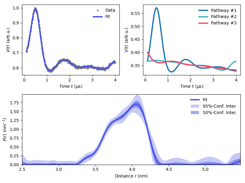
Analysis of a 4-pulse DEER signal with multiple dipolar pathways

Fit a 4-pulse DEER with multiple dipolar pathways and display the individual pathway contributions.

import numpy as np
import matplotlib.pyplot as plt
import deerlab as dl

# File location
path = '../data/'
file = 'example_4pdeer_2.DTA'

# Experimental parameters
tau1 = 0.5      # First inter-pulse delay, μs
tau2 = 3.5      # Second inter-pulse delay, μs
tmin = 0.1  # Start time, μs

# Load the experimental data
t,Vexp = dl.deerload(path + file)

# Pre-processing
Vexp = dl.correctphase(Vexp) # Phase correction
Vexp = Vexp/np.max(Vexp)     # Rescaling (aesthetic)
t = t - t[0]                     # Account for zerotime
t = t + tmin
# Distance vector
r = np.arange(2.5,5.5,0.025) # nm

# Construct the model
experiment = dl.ex_4pdeer(tau1,tau2, pathways=[1,2,3])
Vmodel = dl.dipolarmodel(t,r,experiment=experiment)

# Fit the model to the data
results = dl.fit(Vmodel,Vexp)

# Print results summary
print(results)

Goodness-of-fit:
========= ============= ============= ===================== =======
 Dataset   Noise level   Reduced 𝛘2    Residual autocorr.    RMSD
========= ============= ============= ===================== =======
   #1         0.005         1.172             0.043          0.005
========= ============= ============= ===================== =======
Model hyperparameters:
==========================
 Regularization parameter
==========================
          0.078
==========================
Model parameters:
=========== ======== ========================= ====== ======================================
 Parameter   Value    95%-Confidence interval   Unit   Description
=========== ======== ========================= ====== ======================================
 lam1        0.307    (0.302,0.313)                    Amplitude of pathway #1
 reftime1    0.498    (0.491,0.504)              μs    Refocusing time of pathway #1
 lam2        0.056    (0.048,0.064)                    Amplitude of pathway #2
 reftime2    3.985    (3.958,4.012)              μs    Refocusing time of pathway #2
 lam3        0.069    (0.042,0.097)                    Amplitude of pathway #3
 reftime3    -0.045   (-0.048,0.048)             μs    Refocusing time of pathway #3
 conc        97.921   (81.454,114.387)           μM    Spin concentration
 P           ...      (...,...)                 nm⁻¹   Non-parametric distance distribution
 P_scale     1.177    (1.176,1.179)             None   Normalization factor of P
=========== ======== ========================= ====== ======================================

# Extract fitted dipolar signal
Vfit = results.model

# Extract fitted distance distribution
Pfit = results.P
Pci95 = results.PUncert.ci(95)
Pci50 = results.PUncert.ci(50)

plt.figure(figsize=[8,6])
violet = '#4550e6'
green = '#3cb4c6'
red = '#f84862'
plt.subplot(221)
# Plot experimental data
plt.plot(t,Vexp,'.',color='grey',label='Data')
# Plot the fitted signal
plt.plot(t,Vfit,linewidth=3,color=violet,label='Fit')
plt.legend(frameon=False,loc='best')
plt.xlabel('Time $t$ (μs)')
plt.ylabel('$V(t)$ (arb.u.)')

plt.subplot(222)
lams = [results.lam1, results.lam2, results.lam3]
reftimes = [results.reftime1, results.reftime2, results.reftime3]
colors= ['tab:blue',green, red]
Vinter = results.P_scale*(1-np.sum(lams))*np.prod([dl.bg_hom3d(t-reftime,results.conc,lam) for lam,reftime in zip(lams,reftimes)],axis=0)
for n,(lam,reftime,color) in enumerate(zip(lams,reftimes,colors)):
    Vpath = (1-np.sum(lams) + lam*dl.dipolarkernel(t-reftime,r)@Pfit)*Vinter
    plt.plot(t,Vpath,linewidth=3,label=f'Pathway #{n+1}',color=color)
plt.legend(frameon=False,loc='best')
plt.xlabel('Time $t$ (μs)')
plt.ylabel('$V(t)$ (arb.u.)')

# Plot the distance distribution
plt.subplot(212)
plt.plot(r,Pfit,linewidth=3,color=violet,label='Fit')
plt.fill_between(r,Pci95[:,0],Pci95[:,1],alpha=0.3,color=violet,label='95%-Conf. Inter.',linewidth=0)
plt.fill_between(r,Pci50[:,0],Pci50[:,1],alpha=0.5,color=violet,label='50%-Conf. Inter.',linewidth=0)
plt.legend(frameon=False,loc='best')
plt.autoscale(enable=True, axis='both', tight=True)
plt.xlabel('Distance $r$ (nm)')
plt.ylabel('$P(r)$ (nm$^{-1}$)')

plt.tight_layout()
plt.show()