Analysis of a 6-pulse DQC signal with multiple dipolar pathways

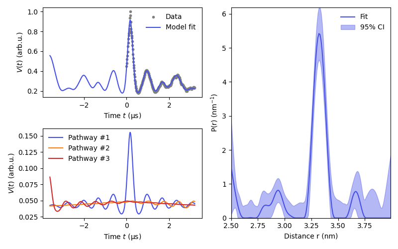
Fit an experimental 6-pulse DQC signal with a model with a non-parametric distribution and a homogeneous background, using Tikhonov regularization. The model assumes three dipolar pathways (#1, #2, and #3) to be contributing to the data.

import numpy as np
import deerlab as dl
import matplotlib.pyplot as plt
violet = '#4550e6'

# Load experimental data
file = '../data/experimental_dqc_1.DTA'
t,Vexp = dl.deerload(file)

# Experimental parameters
tau2 = 2.0 # μs
tau1 = 1.8 # μs
tau3 = 0.2 # μs

# Pre-processing
Vexp = dl.correctphase(Vexp)
t = t-t[0]

# Remove data outside of the detectable range
Vexp = Vexp[t<=2*tau2-4*tau3]
t = t[t<=2*tau2-4*tau3]

# Mask out artificial spike due to spectrometer issue
mask = (t<0.05) | (t>0.15)
Vexp = Vexp/max(Vexp[mask])

# Construct the model
r = np.arange(2.5,4,0.01) # nm
experiment = dl.ex_dqc(tau1,tau2,tau3,pathways=[1,2,3])
Vmodel =  dl.dipolarmodel(t,r,experiment=experiment)

# The amplitudes of the second and third pathways must be equal
Vmodel = dl.link(Vmodel,lam23=['lam2','lam3'])

# Fit the model to the data
results = dl.fit(Vmodel,Vexp,mask=mask)

# Display a summary of the results
print(results)

Goodness-of-fit:
========= ============= ============== ===================== =======
 Dataset   Noise level    Reduced 𝛘2    Residual autocorr.    RMSD
========= ============= ============== ===================== =======
   #1         0.003         21.555             1.593          0.012
========= ============= ============== ===================== =======
Model hyperparameters:
==========================
 Regularization parameter
==========================
          0.046
==========================
Model parameters:
=========== ========= ========================= ====== ======================================
 Parameter   Value     95%-Confidence interval   Unit   Description
=========== ========= ========================= ====== ======================================
 lam1        0.395     (0.366,0.423)                    Amplitude of pathway #1
 reftime1    0.168     (0.165,0.172)              μs    Refocusing time of pathway #1
 lam23       0.213     (0.191,0.236)                    Amplitude of pathway #2
 reftime2    3.952     (3.952,4.015)              μs    Refocusing time of pathway #2
 reftime3    -3.648    (-3.648,-3.552)            μs    Refocusing time of pathway #3
 conc        104.854   (71.059,138.649)           μM    Spin concentration
 P           ...       (...,...)                 nm⁻¹   Non-parametric distance distribution
 P_scale     1.803     (1.780,1.825)             None   Normalization factor of P
=========== ========= ========================= ====== ======================================

# Plot the results
plt.figure(figsize=[8,5])

# Plot the full detectable range
tfull = np.arange(-2*tau1,2*tau2-4*tau3,0.008)
Vmodelext =  dl.dipolarmodel(tfull,r,experiment=experiment)
Vmodelext = dl.link(Vmodelext,lam23=['lam2','lam3'])

# Extract results
Pfit = results.P
Pci = results.PUncert.ci(95)
lams = [results.lam1, results.lam23, results.lam23]
reftimes = [results.reftime1, results.reftime2, results.reftime3]
colors= [violet,'tab:orange','tab:red']

# Plot the data and fit
plt.subplot(221)
plt.plot(t,Vexp,'.',color='grey',label='Data')
plt.plot(tfull,results.evaluate(Vmodelext),color=violet,label='Model fit')
plt.legend(frameon=False,loc='best')
plt.xlabel('Time $t$ (μs)')
plt.ylabel('$V(t)$ (arb.u.)')

# Plot the individual pathway contributions
plt.subplot(223)
Vinter = results.P_scale*(1-np.sum(lams))*np.prod([dl.bg_hom3d(tfull-reftime,results.conc,lam) for lam,reftime in zip(lams,reftimes)],axis=0)
for n,(lam,reftime,color) in enumerate(zip(lams,reftimes,colors)):
    Vpath = (1-np.sum(lams) + lam*dl.dipolarkernel(tfull-reftime,r)@Pfit)*Vinter
    plt.plot(tfull,Vpath,label=f'Pathway #{n+1}',color=color)
plt.legend(frameon=False,loc='best')
plt.xlabel('Time $t$ (μs)')
plt.ylabel('$V(t)$ (arb.u.)')

# Plot the distance distribution
plt.subplot(122)
plt.plot(r,Pfit,color=violet,label='Fit')
plt.fill_between(r,*Pci.T,color=violet,alpha=0.4,label='95% CI')
plt.legend(frameon=False,loc='best')
plt.xlabel('Distance r (nm)')
plt.ylabel('P(r) (nm$^{-1}$)')
plt.autoscale(enable=True, axis='both', tight=True)

plt.tight_layout()
plt.show()