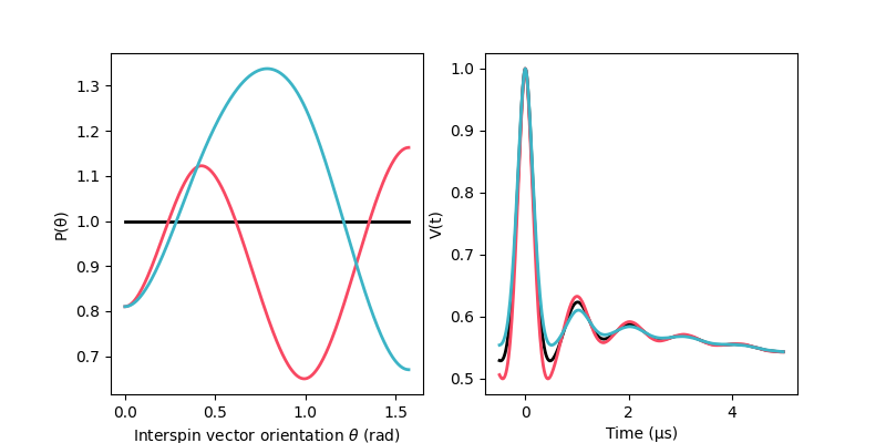
Simulating orientation selection effects in dipolar signals

An example on how to simulate dipolar signals with orientation selection effects.

Specifically, we simulate a dipolar signal with orientation selection effects arising from three different distributions of the orientation weights for a 4-pulse DEER dipolar signal simulated from a worm-like chain (WLC) distance distribution.

The orientation weights distributions are modelled as a 4-point spline with zero-derivative.

# Import the required libraries
import numpy as np
import matplotlib.pyplot as plt
import deerlab as dl
from scipy.interpolate import make_interp_spline

# Simulation parameters
reftime = 0         # Refocusing time, μs
conc = 50           # Spin concentration, μM
moddepth = 0.4      # Modulation depth
contour = 4.0       # Contour length, nm
persistence = 5.0   # Persistence length, nm
rmin,rmax = 1.5,6   # Range of the distance axis, nm
Δr = 0.050          # Distance resolution, nm
tmin,tmax = -0.5,5  # Range of the time trace, μs
Δt = 0.016          # Time resolution, μs

# Experimental time vector
t = np.arange(tmin,tmax,Δt)
# Distance vector
r = np.arange(rmin,rmax,Δr)

# Orientation selection distribution (must be a function defined in the range θ=[0,pi/2])
def Pθ_fcn(θ,Pθspline):
    splineθ = [0, 0.4, 1, np.pi/2]
    # Model P(θ) as a 4-point spline with zero-derivative at the edges
    Pθ = make_interp_spline(splineθ, Pθspline, bc_type='clamped')
    return 1-Pθ(θ)

# Spline parameters for the orientation selection distribution
spline_parameters = [
    [0, 0, 0, 0],                   # Uniform, no orientation selection
    [0.19, -0.12, 0.35, -0.163],    # Least weighted θ=1
    [0.19, -0.12, -0.25, 0.33]      # Least weighted θ=0 and θ=pi/2
]

# Prepare the figure and axes
plt.figure(figsize=[8,4])
ax1 = plt.subplot(121)
ax2 = plt.subplot(122)
# Define custom colors for the plot
black = '#000000'
green = '#3cb4c6'
red = '#f84862'
colors = [black,red,green]

# Loop over the three cases
for spline_param,color in zip(spline_parameters,colors):

    # Define the orientation selection distribution function
    Porisel = lambda θ: Pθ_fcn(θ, spline_param)

    # Construct the dipolar signal model
    Vmodel = dl.dipolarmodel(t,r,Pmodel=dl.dd_wormchain,orisel=Porisel)

    # Simulate the signal with orientation selection
    Vsim = Vmodel(contour=contour, persistence=persistence, reftime=reftime, mod=moddepth, conc=conc, scale=1)

    # Plot the simulated orientation selection distribution
    θ = np.linspace(0,np.pi/2,300)
    ax1.plot(θ,Porisel(θ),color=color,lw=2)
    # Plot the simulated signal
    ax2.plot(t,Vsim,color=color,lw=2)

# Format the figure
ax1.set_xlabel('Interspin vector orientation $θ$ (rad)')
ax1.set_ylabel('P(θ)')
ax2.set_xlabel('Time (μs)')
ax2.set_ylabel('V(t)')
plt.show()