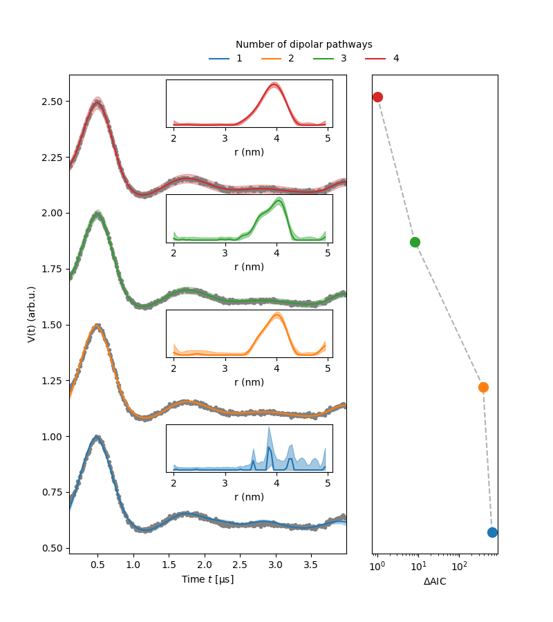
Dipolar pathways model selection

An example on how to select the number of dipolar pathways to include in the model based on the Akaike information criterion.

# Import the required libraries
import numpy as np
import matplotlib.pyplot as plt
from matplotlib.gridspec import GridSpec
from mpl_toolkits.axes_grid1.inset_locator import inset_axes, InsetPosition
import deerlab as dl

# File location
path = '../data/'
file = 'example_4pdeer_2.DTA'

# Experimental parameters
tau1 = 0.5      # First inter-pulse delay, μs
tau2 = 3.5      # Second inter-pulse delay, μs
tmin = 0.1      # Start time, μs

# Load the experimental data
t,Vexp = dl.deerload(path + file)

# Pre-processing
Vexp = dl.correctphase(Vexp) # Phase correction
Vexp = Vexp/np.max(Vexp)     # Rescaling (aesthetic)
t = t - t[0]                 # Account for zerotime
t = t + tmin
# Construct the distance vector
r = np.arange(2,5,0.05)

# 4-pulse DEER can have up to four different dipolar pathways
Nmax = 4

# Create the 4-pulse DEER signal models with increasing number of pathways
Vmodels = [dl.dipolarmodel(t, r, experiment=dl.ex_4pdeer(tau1,tau2,pathways=np.arange(n+1)+1)) for n in range(Nmax)]

# Fit the individual models to the data
fits = [[] for _ in range(Nmax)]
for n,Vmodel in enumerate(Vmodels):
    fits[n] = dl.fit(Vmodel,Vexp)

# Extract the values of the Akaike information criterion for each fit
aic = np.array([fit.stats['aic'] for fit in fits])
# Compute the relative difference in AIC
aic = aic - aic.min() + 1 # ...add plus one for log-scale

# Plotting
colors = ['tab:blue','tab:orange','tab:green','tab:red']
fig = plt.figure(figsize=[8,9])
gs = GridSpec(1, 3, figure=fig)
ax1 = fig.add_subplot(gs[0, :-1])
for n in range(len(Vmodels)):
    # Get the fits of the dipolar signal models
    Vfit = fits[n].model
    # Get the confidence intervals of the dipolar signal models
    Vci = fits[n].propagate(Vmodels[n]).ci(95)
    # Plot the experimental data
    ax1.plot(t,n/2+Vexp,'.',color='grey')
    # Plot the dipolar signal fits and their confidence bands
    ax1.plot(t,n/2 + Vfit,label=f'{1+n}',linewidth=1.5,color=colors[n])
    ax1.fill_between(t,n/2+Vci[:,0],n/2+Vci[:,1],alpha=0.3,color=colors[n])

# Plot the distance distributions as insets
for n in range(Nmax):
    # Get the distance distribution and its confidence intervals
    Pfit = fits[n].P
    Pci = fits[n].PUncert.ci(95)
    # Setup the inset plot
    axins = inset_axes(ax1,width="30%", height="30%", loc='upper left')
    ip = InsetPosition(ax1,[0.35, 0.17+0.24*n, 0.6, 0.1])
    axins.set_axes_locator(ip)
    axins.yaxis.set_ticklabels([])
    axins.yaxis.set_visible(False)
    # Plot the distance distributions and their confidence bands
    axins.plot(r,Pfit,color=colors[n])
    axins.fill_between(r,Pci[:,0],Pci[:,1],alpha=0.4,color=colors[n])
    axins.set_xlabel('r (nm)')

# Plot the difference in AIC for each fit
ax2 = fig.add_subplot(gs[0,-1])
ax2.plot(aic,np.arange(Nmax),'k--',alpha=0.3)
for n in range(Nmax):
    ax2.semilogx(aic[n],n,'o',markersize=10)
ax2.yaxis.set_visible(False)

# Axes settings
ax1.set_ylabel('V(t) (arb.u.)')
ax1.set_xlabel('Time $t$ [μs]')
ax1.autoscale(enable=True, axis='x', tight=True)
ax2.set_xlabel('$\Delta$AIC')
ax2.yaxis.set_ticklabels([])

# Legend settings
handles, labels = ax1.get_legend_handles_labels()
fig.legend(handles, labels, title='Number of dipolar pathways', frameon=False,
            loc='upper center',ncol=Nmax,bbox_to_anchor=(0.55, 0.95))
plt.show()

/home/runner/work/DeerLab/DeerLab/examples/advanced/ex_dipolarpathways_selection.py:83: MatplotlibDeprecationWarning: The InsetPosition class was deprecated in Matplotlib 3.8 and will be removed two minor releases later. Use Axes.inset_axes instead.
  ip = InsetPosition(ax1,[0.35, 0.17+0.24*n, 0.6, 0.1])
/home/runner/work/DeerLab/DeerLab/examples/advanced/ex_dipolarpathways_selection.py:83: MatplotlibDeprecationWarning: The InsetPosition class was deprecated in Matplotlib 3.8 and will be removed two minor releases later. Use Axes.inset_axes instead.
  ip = InsetPosition(ax1,[0.35, 0.17+0.24*n, 0.6, 0.1])
/home/runner/work/DeerLab/DeerLab/examples/advanced/ex_dipolarpathways_selection.py:83: MatplotlibDeprecationWarning: The InsetPosition class was deprecated in Matplotlib 3.8 and will be removed two minor releases later. Use Axes.inset_axes instead.
  ip = InsetPosition(ax1,[0.35, 0.17+0.24*n, 0.6, 0.1])
/home/runner/work/DeerLab/DeerLab/examples/advanced/ex_dipolarpathways_selection.py:83: MatplotlibDeprecationWarning: The InsetPosition class was deprecated in Matplotlib 3.8 and will be removed two minor releases later. Use Axes.inset_axes instead.
  ip = InsetPosition(ax1,[0.35, 0.17+0.24*n, 0.6, 0.1])