Fitting#

Fitting the model#

The model Vmodel can be fitted to the experimental data V by calling the fit function:

result = dl.fit(Vmodel,Vexp)  # Fit the model to the experimental data

After fit has found a solution, it returns an object that we assigned to result. This object contains fields with all quantities of interest with the fit results, such as the fitted model and parameters, goodness-of-fit statistics, and uncertainty information. Check out the fitting guide for more details on the quantities provided in result.

Adding penalties#

Penalty terms can be added to the objective function to impose certain properties upon the solution. While DeerLab can take any kind of penalty function (see the fitting guide for details), for dipolar models it provides a specialized function dipolarpenalty which easily generates penalties based on the distance distribution.

To generate such a penalty, you must provide the model Pmodel for the distance distribution (as provided in dipolarmodel), as well as the distance axis vector r. Next, the type of penalty must be specified:

'compactness': Imposes compactness of the distance distribution. A compact distribution avoid having distribution mass spread towards the edges of the distance axis vector.
'smoothness': Imposes smoothness of the distance distribution. This is particularly useful for imposing smoothness of parametric models of the distance distribution. For non-parametric distributions, smoothness is already imposed by the regularization criterion, making this penalty unnecessary.

All penalties are weighted by a weighting parameter, which is optimized according to a selection criterion which must be specified to the dipolarpenalty method. For the smoothness penalty, the 'aic' criterion is recommended, while for the smoothness criterion, the 'icc' criterion is recommended.

The dipolarpenalty function will return a Penalty object which can be passed to the fit function through the penalties keyword argument.

Example: Fitting a non-parametric distribution with a compactness criterion#

For example, to introduce compactness in the fit of a dipolar model with a non-parametric distance distribution we must set the distribution model to None to indicate a non-parametric distribution

compactness_penalty = dl.dipolarpenalty(None, r, 'compactness', 'icc')
results = dl.fit(Vmodel,Vexp, penalties=compactness_penalty)

Example: Fitting a Gaussian distribution with a compactness criterion#

For example, to introduce compactness in the fit of a dipolar model with a Gaussian distance distribution we must set the distribution model to dd_gauss to indicate the parametric distribution

compactness_penalty = dl.dipolarpenalty(dl.dd_gauss, r, 'compactness', 'icc')
results = dl.fit(Vmodel,Vexp, penalties=compactness_penalty)

Displaying the results#

For just a quick display of the results, you can use the plot() method of the fit object that will display a figure with you experimental data, the corresponding fit including confidence bands.

results.plot(axis=t,xlabel='Time (μs)') # display results

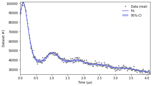
For a quick summary of the fit results, including goodness-of-fit statistics, used model hyperparameters, and the fitted model parameter values (including 95% confidence intervals), can be accessed by just printing the results object:

>>>print(results)
Goodness-of-fit:
========= ============= ============ ==================== ==========
 Dataset   Noise level   Reduced 𝛘2   Residual autocorr.     RMSD
========= ============= ============ ==================== ==========
   #1       1426.905       1.036            0.127          1443.706
========= ============= ============ ==================== ==========

Model hyperparameters:
========================== ===================
 Regularization parameter   Penalty weight #1
========================== ===================
        0.002                   0.060
========================== ===================

Model parameters:
=========== ========= ========================= ======= ======================================
 Parameter   Value     95%-Confidence interval   Units   Description
=========== ========= ========================= ======= ======================================
 mod         0.505     (0.494,0.516)                     Modulation depth
 reftime     0.096     (0.092,0.100)              μs     Refocusing time
 conc        295.909   (279.412,312.405)          μM     Spin concentration
 P           ...       (...,...)                 None    Non-parametric distance distribution
 P_scale     1.001e5                             None    Normalization factor of P
=========== ========= ========================= ======= ======================================

The first table contains all the goodness-of-fit statistics (see below). The second table summarizes all the hyperparameters used in the final evaluation of the model. If regularization is enabled (as is the case when using non-parametric distance distributions) its final value will be shown. If additional penalties have been added to the fit, their regularization parameters (i.e. penalty weights) will be shown as well.

The third table summarizes all the model parameter estimates along with their uncertainties and model descriptions. The values of vectorized parameters such as P are not shown in this summary and shown instead as .... The additional value P_scale corresponds to the overall scaling factor of the distance distribution (and hence of the dipolar signal) since the fitted distance distribution is normalized such that trapz(P,r)==1.

Any specific quantities can be extracted from the results object. For each parameter in the model, the results output contains an attribute results.<parameter> named after the parameter containing the fitted value of that parameter, as well as another attribute results.<parameter>Uncert containing the uncertainty estimates of that parameter, from which confidence intervals can be constructed (the uncertainty guide for details). For example:

# Distance distribution
results.P # Fitted distance distribution
results.PUncert.ci(95) # Distance distribution 95% confidence intervals

# Modulation depth
results.mod # Fitted modulation depth
results.modUncert.ci(95) # Modulation depth 95% confidence intervals

Assessing the goodness-of-fit#

The results summary shown above contains several key quantities to quickly assess whether the model estimate obtained by the fit function is a proper descriptor of the data. For each dataset analyzed, several quantities are returned. The Noise level value shows either the estimated noise level of that dataset or the one specified by the user. The Reduced 𝛘2 value indicates how good the model fit describes the data. Values close to 1 indicate a good fit of the data. The Residual autocorr. value (computed as $\vert 2 - d_\mathrm{DW} \vert$ , where $d_\mathrm{DW}$ is the Durbin–Watson statistic) indicates the degree of (first-order) autocorrelation in the fit residual. Values larger than 0.5 indicate a significant amount of autocorrelation, meaning that either the noise if not independent or that the model might not have fully captured all features in the data. Such autocorrelation con commonly originate from a simplified distance distribution model failing to capture all dipolar modulations or a insufficient set of dipolar pathways that fail to capture all contributions to the data. The RMSD value does not provide any insight by itself, however, it can be used to compare the goodness-of-fit between different models.

To facilitate the inspection of the goodness-of-fit, DeerLab will highlight those values that indicate a potential failure of the analysis. If either or both the Reduced 𝛘2 or Residual autocorr. values are highlighted in yellow, it will indicate that there is a significant possibility that the model does not properly describe the data. In such cases, one must inspect, e.g. visually using results.plot(gof=True) (see here for details), whether the model estimate actually is a good descriptor of the data. If the values are shown in red, it will indicate that the model does certainly not properly describe the data.

If yellow or red goodness-of-fit quantities are obtained after an analysis, the following steps can be taken to amend that:

Check for outliers or features in the data not accounted for by the model.
Expand the model to account for them or approximate their presence.
If the model cannot be expanded to account for them, make use of the fit function’s masks optional argument to specify data masks so that those features are not accounted for during the analysis.

Exporting the figure and the data#

After completing the fit, you might want to export the figure with the fit. Here is one way to do it:

figure = fit.plot()                       # get figure object
figure.savefig('DEERFig.png', dpi=600)    # save figure as png file
figure.savefig('DEERFig.pdf')             # save figure as pdf file

To export the fitted distance distribution for plotting with another software, save it in a simple text file

np.savetxt('distancedistribution.txt', np.asarray((r, fit.P, *fit.Puncert.ci(95).T)).T)

The generated file contain four columns: the distance axis, the distance distributions, and the upper and lower confidence bounds. The .T indicate array transposes, which are used to get the confidence bands into the column format for saving.

To export the fitted time-domain trace, use similarly

np.savetxt('timetrace.txt', np.asarray((t, V, fit.V, *fit.Vuncert.ci(95).T)).T)