Analyzing data with crossing echoes robustly

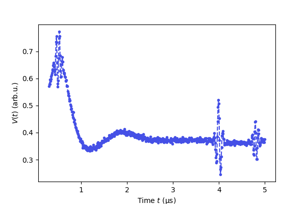
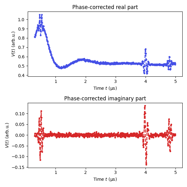
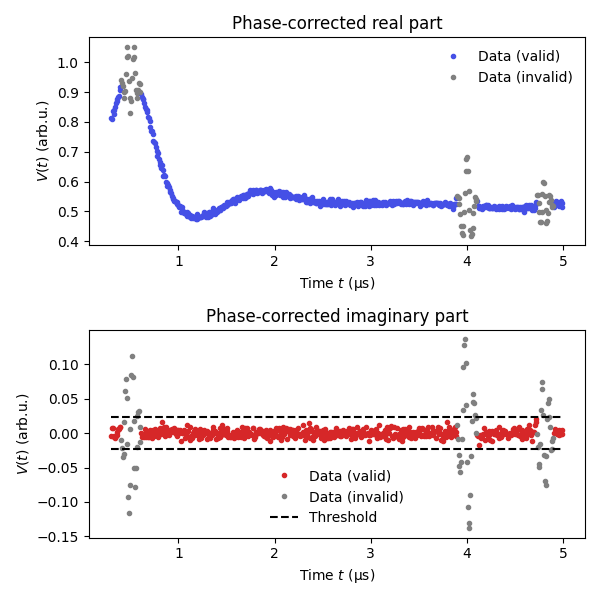
How to deal with the presence of crossing echoes in the data. Crossing echoes appear as spurious peaks/oscillations in the data that cannot be accounted for by the model constructed by dipolarmodel(). Their presence will thus distort the analysis and lead to incorrect results. To be able to analyze such datasets robustly DeerLab allows the definition of masks, i.e. a list of True (keep data point) and False (ignore data point) values, to remove their influence during the fit procedure without the need to remove them from the data or the model. For crossing echoes, we can define such a mask robustly since their presence also affect the imaginary part of the data, and we know that the imaginary part of the data should only contain white noise. We can define a mask that ignores those data points whose imaginary part value exceeds several multiples of the expected noise level in the data. Once such a mask is constructed, the analysis can be executed as usual without any additional modifications.

# Import the required libraries
import numpy as np
import matplotlib.pyplot as plt
import deerlab as dl
violet = '#4550e6'

# Load the experimental data
t,Vexp = dl.deerload('../data/example_4pdeer_5.DTA')

t *= 1e3 # convert from ms to us

# Experimental parameters
tau1 = 0.5  # First inter-pulse time delay, μs
tau2 = 4.5  # Second inter-pulse time delay, μs
tmin = 0.3    # Start time, μs

t = t - t[0]                     # Account for zerotime
t = t + tmin

# Plot the real part of the raw data
plt.figure(figsize=[6,4])
plt.plot(t,Vexp.real,'.--',color=violet)
plt.xlabel('Time $t$ (μs)')
plt.ylabel('$V(t)$ (arb.u.)')
plt.show()

# Perform phase correction, returning the phase-corrected imaginary part
Vexp,Vim,_ = dl.correctphase(Vexp, full_output=True, offset=True)

# Plot the phase corrected data
plt.figure(figsize=[6,6])
plt.subplot(211)
plt.plot(t,Vexp,'.--',lw=2,color=violet)
plt.xlabel('Time $t$ (μs)')
plt.ylabel('$V(t)$ (arb.u.)')
plt.title('Phase-corrected real part')
plt.subplot(212)
plt.plot(t,Vim,'.--',lw=2,color='tab:red')
plt.xlabel('Time $t$ (μs)')
plt.ylabel('$V(t)$ (arb.u.)')
plt.title('Phase-corrected imaginary part')
plt.tight_layout()
plt.show()

# Estimate the noise level in the data
noiselevel = dl.noiselevel(Vim)
# Define the threshold for crossing echo outliers (some multiple of the noise level)
masking_threshold = 4*noiselevel

# Construct the mask for the data, exclude data points
# corresponding to the crossing echoes
mask = abs(Vim)<masking_threshold # Mask[i]=True implies that the i-th data point is valid

# (Optional)
# Mask out also two points around those already masked out to ensure
# all influence of the crossing echoes is removed
n = 2
mask[np.where(~mask)[0]-n] = False
mask[np.where(~mask)[0]+n] = False

# Plot the masking
plt.figure(figsize=[6,6])
plt.subplot(211)
plt.plot(t[mask],Vexp[mask],'.',lw=2,color=violet,label='Data (valid)')
plt.plot(t[~mask],Vexp[~mask],'.',lw=2,color='grey',label='Data (invalid)')
plt.xlabel('Time $t$ (μs)')
plt.ylabel('$V(t)$ (arb.u.)')
plt.title('Phase-corrected real part')
plt.legend(frameon=False,loc='best')
plt.subplot(212)
plt.plot(t[mask],Vim[mask],'.',lw=2,color='tab:red',label='Data (valid)')
plt.plot(t[~mask],Vim[~mask],'.',lw=2,color='grey',label='Data (invalid)')
plt.xlabel('Time $t$ (μs)')
plt.ylabel('$V(t)$ (arb.u.)')
plt.title('Phase-corrected imaginary part')
plt.hlines(masking_threshold,min(t),max(t),color='k',linestyles='dashed',label='Threshold')
plt.hlines(-masking_threshold,min(t),max(t),color='k',linestyles='dashed')
plt.legend(frameon=False,loc='best')
plt.tight_layout()
plt.show()

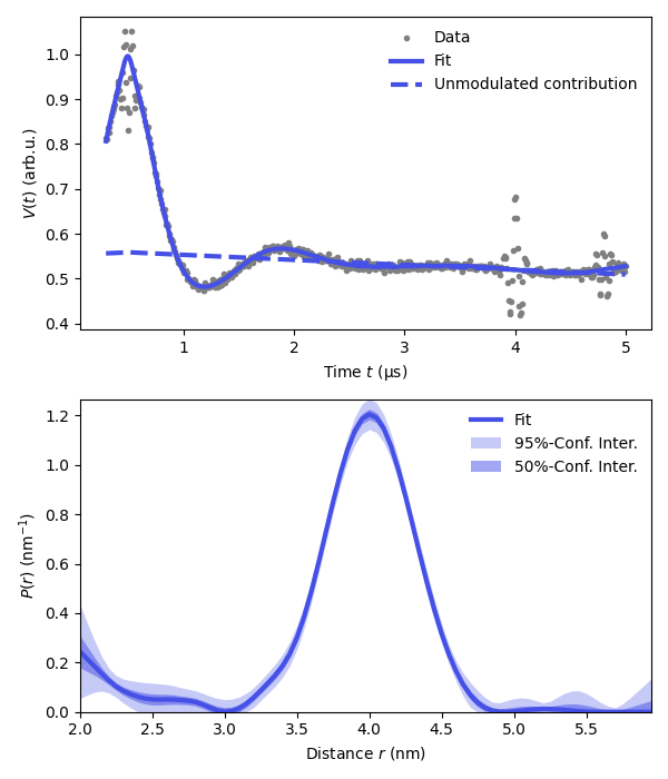
# Distance vector
r = np.arange(2,6,0.05) # nm

# Construct the dipolar signal model
experiment = dl.ex_4pdeer(tau1,tau2,pathways=[1,2,3])
Vmodel = dl.dipolarmodel(t,r,experiment=experiment)

# Analyze the data while ignoring the crossing echoes
results = dl.fit(Vmodel,Vexp, mask=mask, noiselvl=noiselevel)

# Display summary of fit results
print(results)

Goodness-of-fit:
========= ============= ============= ===================== =======
 Dataset   Noise level   Reduced 𝛘2    Residual autocorr.    RMSD
========= ============= ============= ===================== =======
   #1         0.006         0.922             0.034          0.005
========= ============= ============= ===================== =======
Model hyperparameters:
==========================
 Regularization parameter
==========================
          0.275
==========================
Model parameters:
=========== ========== ========================= ====== ======================================
 Parameter   Value      95%-Confidence interval   Unit   Description
=========== ========== ========================= ====== ======================================
 lam1        0.429      (0.380,0.479)                    Amplitude of pathway #1
 reftime1    0.496      (0.481,0.512)              μs    Refocusing time of pathway #1
 lam2        0.021      (0.013,0.028)                    Amplitude of pathway #2
 reftime2    5.024      (4.952,5.048)              μs    Refocusing time of pathway #2
 lam3        5.52e-04   (0.00e+00,0.127)                 Amplitude of pathway #3
 reftime3    -0.033     (-0.048,0.048)             μs    Refocusing time of pathway #3
 conc        50.413     (37.171,63.656)            μM    Spin concentration
 P           ...        (...,...)                 nm⁻¹   Non-parametric distance distribution
 P_scale     1.022      (1.021,1.023)             None   Normalization factor of P
=========== ========== ========================= ====== ======================================

# Extract fitted dipolar signal
Vfit = results.model

# Extract fitted distance distribution
Pfit = results.P
Pci95 = results.PUncert.ci(95)
Pci50 = results.PUncert.ci(50)

# Extract the unmodulated contribution
def Vunmodfcn(lam1,lam2,lam3,reftime1,reftime2,reftime3,conc):
    Lam0 = results.P_scale*(1-lam1-lam2-lam3)
    Vunmod = Lam0*dl.bg_hom3d(t-reftime1,conc,lam1)
    Vunmod *= dl.bg_hom3d(t-reftime2,conc,lam2)
    Vunmod *= dl.bg_hom3d(t-reftime3,conc,lam3)
    return Vunmod
Bfit = results.evaluate(Vunmodfcn)

plt.figure(figsize=[6,7])
violet = '#4550e6'
plt.subplot(211)
# Plot experimental and fitted data
plt.plot(t,Vexp,'.',color='grey',label='Data')
plt.plot(t,Vfit,linewidth=3,color=violet,label='Fit')
plt.plot(t,Bfit,'--',linewidth=3,color=violet,label='Unmodulated contribution')
plt.legend(frameon=False,loc='best')
plt.xlabel('Time $t$ (μs)')
plt.ylabel('$V(t)$ (arb.u.)')
# Plot the distance distribution
plt.subplot(212)
plt.plot(r,Pfit,color=violet,linewidth=3,label='Fit')
plt.fill_between(r,Pci95[:,0],Pci95[:,1],alpha=0.3,color=violet,label='95%-Conf. Inter.',linewidth=0)
plt.fill_between(r,Pci50[:,0],Pci50[:,1],alpha=0.5,color=violet,label='50%-Conf. Inter.',linewidth=0)
plt.legend(frameon=False,loc='best')
plt.autoscale(enable=True, axis='both', tight=True)
plt.xlabel('Distance $r$ (nm)')
plt.ylabel('$P(r)$ (nm$^{-1}$)')
plt.tight_layout()
plt.show()