Analysing the selection of regularisation parameter

This example demonstates how to generate plots from the regularisation parameter selection, and how to use this infomation.

import numpy as np
import matplotlib.pyplot as plt
import deerlab as dl

# File location
path = '../data/'
file = 'example_4pdeer_1.DTA'

# Experimental parameters
tau1 = 0.3      # First inter-pulse delay, μs
tau2 = 4.0      # Second inter-pulse delay, μs
tmin = 0.1      # Start time, μs

# Load the experimental data
t,Vexp = dl.deerload(path + file)

# Pre-processing
Vexp = dl.correctphase(Vexp) # Phase correction
Vexp = Vexp/np.max(Vexp)     # Rescaling (aesthetic)
t = t - t[0]                     # Account for zerotime
t = t + tmin

# Distance vector
r = np.linspace(1.5,7,100) # nm

# Construct the model
Vmodel = dl.dipolarmodel(t,r, experiment=dl.ex_4pdeer(tau1,tau2, pathways=[1]))

# Fit the model to the data with compactness criterion
results= dl.fit(Vmodel,Vexp,regparam='bic')
print(results)

Goodness-of-fit:
========= ============= ============= ===================== =======
 Dataset   Noise level   Reduced 𝛘2    Residual autocorr.    RMSD
========= ============= ============= ===================== =======
   #1         0.005         0.837             0.060          0.004
========= ============= ============= ===================== =======
Model hyperparameters:
==========================
 Regularization parameter
==========================
          0.044
==========================
Model parameters:
=========== ========= ========================= ====== ======================================
 Parameter   Value     95%-Confidence interval   Unit   Description
=========== ========= ========================= ====== ======================================
 mod         0.307     (0.143,0.470)                    Modulation depth
 reftime     0.299     (0.298,0.301)              μs    Refocusing time
 conc        139.616   (0.010,496.456)            μM    Spin concentration
 P           ...       (...,...)                 nm⁻¹   Non-parametric distance distribution
 P_scale     1.000     (0.986,1.015)             None   Normalization factor of P
=========== ========= ========================= ====== ======================================

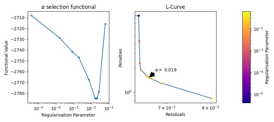
The regularisation parameter in DeerLab can be selected using a variety of criteria. The default criterion is the Akaike complexity criterion (aic) however other criterion exists and can be selected.

Each criterion has its own functional, which is minimised. These functionals are often based on the residuals of the fit vs the raw data, such that a minimal functional value will occur at the location of the best fit. Some methods such as the L-Curve-based methods do not follow this approach.

Traditionally the L-Curve has been used to investigate and select the regularisation parameter. The L-Curve is a plot of the Residual Norm against the Penalty Norm. Each point represents a different regularisation parameter. Normally the optimal regularisation parameter can be found at the kink of the curve, i.e. the place that has both a low Residual Norm and a low Pentalty Norm. Recently, this approach has taken a back foot as the existence of an L-shape or kink is not guaranteed. Nonetheless, it can be useful to diagnose problems in the selection of the regularisation parameter.

fig, axs =plt.subplots(1,3, figsize=(9,4),width_ratios=(1,1,0.1))
alphas = results.regparam_stats['alphas_evaled'][1:]
funcs = results.regparam_stats['functional'][1:]


idx = np.argsort(alphas)

axs[0].semilogx(alphas[idx], funcs[idx],marker='.',ls='-')
axs[0].set_title(r"$\alpha$ selection functional");
axs[0].set_xlabel("Regularisation Parameter")
axs[0].set_ylabel("Functional Value ")

# Just the final L-Curve

cmap = plt.get_cmap('plasma')
import matplotlib as mpl

x = results.regparam_stats['residuals']
y = results.regparam_stats['penalties']
idx = np.argsort(x)


axs[1].loglog(x[idx],y[idx])

n_points = results.regparam_stats['alphas_evaled'].shape[-1]
lams = results.regparam_stats['alphas_evaled']
norm = mpl.colors.LogNorm(vmin=lams[1:].min(), vmax=lams.max())
for i in range(n_points):
    axs[1].plot(x[i], y[i],marker = '.', ms=8, color=cmap(norm(lams[i])))

i_optimal = np.argmin(np.abs(lams - results.regparam))
axs[1].annotate(fr"$\alpha =$ {results.regparam:.2g}", xy = (x[i_optimal],y[i_optimal]),arrowprops=dict(facecolor='black', shrink=0.05, width=5), xytext=(20, 20),textcoords='offset pixels')
fig.colorbar(mpl.cm.ScalarMappable(norm=norm, cmap=cmap),cax=axs[2])
axs[1].set_ylabel("Penalties")
axs[2].set_ylabel("Regularisation Parameter")
axs[1].set_xlabel("Residuals")
axs[1].set_title("L-Curve");
fig.tight_layout()

Over and Under selection of the regularisation parameter

Here we will demonstrate the effect of selecting a regularisation parameter that is either too small or too large.

result_high= dl.fit(Vmodel,Vexp,regparam=1.0)

result_low= dl.fit(Vmodel,Vexp,regparam=1e-4)

green = '#3cb4c6'
red = '#f84862'
fig, axs =plt.subplots(1,2, figsize=(9,4),width_ratios=(1,1))
fig.tight_layout()

axs[0].set_xlabel("Time $t$ (μs)")
axs[0].set_ylabel('$V(t)$ (arb.u.)')
axs[0].plot(t,Vexp,'.',color='grey',label='Data')
axs[0].plot(t,result_high.model,linewidth=3,color=green,label='High regparam')
axs[0].plot(t,result_low.model,linewidth=3,color=red,label='Low regparam')
axs[0].legend(frameon=False,loc='best')

Pfit_h = result_high.P
Pci95_h = result_high.PUncert.ci(95)

Pfit_l = result_low.P
Pci95_l = result_low.PUncert.ci(95)



axs[1].plot(r,Pfit_h,linewidth=3,color=green,label='High regparam')
axs[1].fill_between(r,Pci95_h[:,0],Pci95_h[:,1],alpha=0.3,color=green,linewidth=0)
axs[1].plot(r,Pfit_l,linewidth=3,color=red,label='Low regparam')
axs[1].fill_between(r,Pci95_l[:,0],Pci95_l[:,1],alpha=0.3,color=red,linewidth=0)
axs[1].set_ylim(0,max([Pfit_h.max(),Pfit_l.max()]))
axs[1].legend(frameon=False,loc='best')
axs[1].set_xlabel('Distance $r$ (nm)')
axs[1].set_ylabel('$P(r)$ (nm$^{-1}$)')

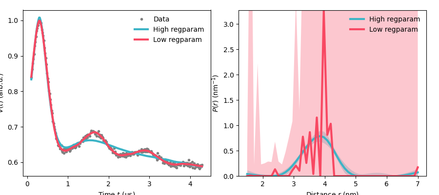
As we can see when the regularisation parameter is too small we still get a high quality fit in the time domain, however, our distance domain data is now way too spikey and non-physical.

# In contrast when the regularisation parameter is too large we struggle to get
# a good fit, however, we get a much smoother distance distribution.
# This could have been seen from the selection functional above. The effect of
# lower regularisation parameter had a smaller effect on the functional than the
# effect of going to a larger one.

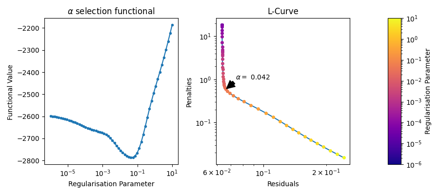
# Plotting the full L-Curve
# ++++++++++++++++++++++++++
# Normally the selection of the regularisation parameter is done through a Brent optimisation
# algorithm. This results in the L-Curve being sparsely sampled. However, the full L-Curve can be
# generated by evaluating the functional at specified regularisation paramters.

# This has the disadvantage of being computationally expensive, however, it can be useful.

regparamrange = 10**np.linspace(np.log10(1e-6),np.log10(1e1),60) # Builds the range of regularisation parameters
results_grid= dl.fit(Vmodel,Vexp,regparam='bic',regparamrange=regparamrange)
print(results_grid)

fig, axs =plt.subplots(1,3, figsize=(9,4),width_ratios=(1,1,0.1))
alphas = results_grid.regparam_stats['alphas_evaled'][:]
funcs = results_grid.regparam_stats['functional'][:]


idx = np.argsort(alphas)

axs[0].semilogx(alphas[idx], funcs[idx],marker='.',ls='-')
axs[0].set_title(r"$\alpha$ selection functional");
axs[0].set_xlabel("Regularisation Parameter")
axs[0].set_ylabel("Functional Value ")

# Just the final L-Curve
x = results_grid.regparam_stats['residuals']
y = results_grid.regparam_stats['penalties']
idx = np.argsort(x)


axs[1].loglog(x[idx],y[idx])

n_points = results_grid.regparam_stats['alphas_evaled'].shape[-1]
lams = results_grid.regparam_stats['alphas_evaled']
norm = mpl.colors.LogNorm(vmin=lams[:].min(), vmax=lams.max())
for i in range(n_points):
    axs[1].plot(x[i], y[i],marker = '.', ms=8, color=cmap(norm(lams[i])))

i_optimal = np.argmin(np.abs(lams - results_grid.regparam))
axs[1].annotate(fr"$\alpha =$ {results_grid.regparam:.2g}", xy = (x[i_optimal],y[i_optimal]),arrowprops=dict(facecolor='black', shrink=0.05, width=5), xytext=(20, 20),textcoords='offset pixels')
fig.colorbar(mpl.cm.ScalarMappable(norm=norm, cmap=cmap),cax=axs[2])
axs[1].set_ylabel("Penalties")
axs[2].set_ylabel("Regularisation Parameter")
axs[1].set_xlabel("Residuals")
axs[1].set_title("L-Curve");
fig.tight_layout()

Goodness-of-fit:
========= ============= ============= ===================== =======
 Dataset   Noise level   Reduced 𝛘2    Residual autocorr.    RMSD
========= ============= ============= ===================== =======
   #1         0.005         0.835             0.065          0.004
========= ============= ============= ===================== =======
Model hyperparameters:
==========================
 Regularization parameter
==========================
          0.042
==========================
Model parameters:
=========== ========= ========================= ====== ======================================
 Parameter   Value     95%-Confidence interval   Unit   Description
=========== ========= ========================= ====== ======================================
 mod         0.308     (0.144,0.472)                    Modulation depth
 reftime     0.299     (0.298,0.301)              μs    Refocusing time
 conc        135.957   (0.010,490.294)            μM    Spin concentration
 P           ...       (...,...)                 nm⁻¹   Non-parametric distance distribution
 P_scale     1.001     (0.986,1.016)             None   Normalization factor of P
=========== ========= ========================= ====== ======================================