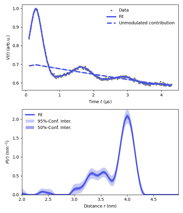
Analysis of a 4-pulse DEER signal with a compactness penalty

Fit a simple 4-pulse DEER signal with a model with a non-parametric distribution and a homogeneous background, using Tikhonov regularization. Additionally, impose compactness of the distance distribution by penalizing for spread of the distance distribution.

import numpy as np
import matplotlib.pyplot as plt
import deerlab as dl

# File location
path = '../data/'
file = 'example_4pdeer_1.DTA'

# Experimental parameters
tau1 = 0.3      # First inter-pulse delay, μs
tau2 = 4.0      # Second inter-pulse delay, μs
tmin = 0.1      # Start time, μs

# Load the experimental data
t,Vexp = dl.deerload(path + file)

# Pre-processing
Vexp = dl.correctphase(Vexp) # Phase correction
Vexp = Vexp/np.max(Vexp)     # Rescaling (aesthetic)
t = t - t[0]                 # Account for zerotime
t = t + tmin

# Distance vector
r = np.arange(2,5,0.025) # nm

# Construct the model
Vmodel = dl.dipolarmodel(t, r, experiment = dl.ex_4pdeer(tau1,tau2, pathways=[1]))
compactness = dl.dipolarpenalty(Pmodel=None, r=r, type='compactness')

# Fit the model to the data
results = dl.fit(Vmodel,Vexp,penalties=compactness)

# Print results summary
print(results)

Goodness-of-fit:
========= ============= ============= ===================== =======
 Dataset   Noise level   Reduced 𝛘2    Residual autocorr.    RMSD
========= ============= ============= ===================== =======
   #1         0.005         0.812             0.125          0.004
========= ============= ============= ===================== =======
Model hyperparameters:
========================== ===================
 Regularization parameter   Penalty weight #1
========================== ===================
          0.070                   0.018
========================== ===================
Model parameters:
=========== ========= ========================= ====== ======================================
 Parameter   Value     95%-Confidence interval   Unit   Description
=========== ========= ========================= ====== ======================================
 mod         0.302     (0.300,0.304)                    Modulation depth
 reftime     0.299     (0.298,0.301)              μs    Refocusing time
 conc        148.111   (144.373,151.850)          μM    Spin concentration
 P           ...       (...,...)                 nm⁻¹   Non-parametric distance distribution
 P_scale     1.000     (0.999,1.000)             None   Normalization factor of P
=========== ========= ========================= ====== ======================================

# Extract fitted dipolar signal
Vfit = results.model

# Extract fitted distance distribution
Pfit = results.P
Pci95 = results.PUncert.ci(95)
Pci50 = results.PUncert.ci(50)

# Extract the unmodulated contribution
Bfcn = lambda mod,conc,reftime: results.P_scale*(1-mod)*dl.bg_hom3d(t-reftime,conc,mod)
Bfit = results.evaluate(Bfcn)
Bci = results.propagate(Bfcn).ci(95)

plt.figure(figsize=[6,7])
violet = '#4550e6'
plt.subplot(211)
# Plot experimental and fitted data
plt.plot(t,Vexp,'.',color='grey',label='Data')
plt.plot(t,Vfit,linewidth=3,color=violet,label='Fit')
plt.plot(t,Bfit,'--',linewidth=3,color=violet,label='Unmodulated contribution')
plt.fill_between(t,Bci[:,0],Bci[:,1],color=violet,alpha=0.3)
plt.legend(frameon=False,loc='best')
plt.xlabel('Time $t$ (μs)')
plt.ylabel('$V(t)$ (arb.u.)')
# Plot the distance distribution
plt.subplot(212)
plt.plot(r,Pfit,color=violet,linewidth=3,label='Fit')
plt.fill_between(r,Pci95[:,0],Pci95[:,1],alpha=0.3,color=violet,label='95%-Conf. Inter.',linewidth=0)
plt.fill_between(r,Pci50[:,0],Pci50[:,1],alpha=0.5,color=violet,label='50%-Conf. Inter.',linewidth=0)
plt.legend(frameon=False,loc='best')
plt.autoscale(enable=True, axis='both', tight=True)
plt.xlabel('Distance $r$ (nm)')
plt.ylabel('$P(r)$ (nm$^{-1}$)')
plt.tight_layout()
plt.show()