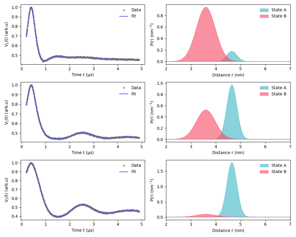
Global fitting of a two-state model to a series of DEER traces

This example shows how to fit a two-state model to a series DEER traces. Each of the two states, A and B, has a one-Gauss distance distribution, and each DEER trace comes from a sample with different fractional populations of the two states. This could be the consequence of a chemical or conformational equilibrium. The model contains global parameters needed for all samples traces (the distribution parameters) and local parameters needed for individual samples traces (the fractional populations).

import numpy as np
import matplotlib.pyplot as plt
import deerlab as dl

green = "#3cb4c6"
red = "#f84862"
violet = "#4550e6"

# File location
path = "../data/"
files = [
    "example_twostate_data_1.DTA",
    "example_twostate_data_2.DTA",
    "example_twostate_data_3.DTA",
]

# Experimental parameters
tau1 = 0.4  # First inter-pulse delay, μs
tau2 = 4.5  # Second inter-pulse delay, μs
tmin = 0.2  # Start time, μs

Vmodels, ts, Vexps = [], [], []
for file in files:

    # Load the experimental data
    t, Vexp = dl.deerload(path + file)

    # Pre-processing
    Vexp = dl.correctphase(Vexp)    # Phase correction
    Vexp = Vexp / np.max(Vexp)      # Rescaling (aesthetic)
    t = t - t[0]                    # Account for zerotime
    t = t + tmin

    # Put the datasets into lists
    ts.append(t)
    Vexps.append(Vexp)

# Define the distance vector
r = np.linspace(2, 7, 200)

# Define a custom distance distribution model function
def Ptwostates(meanA, meanB, stdA, stdB, fracA):
    PA = fracA * dl.dd_gauss(r, meanA, stdA)
    PB = (1 - fracA) * dl.dd_gauss(r, meanB, stdB)
    P = PA + PB
    P /= np.trapz(P)
    return P


# Construct the model object
Pmodel = dl.Model(Ptwostates)
# Set the parameter boundaries and start values
Pmodel.meanA.set(lb=2, ub=7, par0=5)
Pmodel.meanB.set(lb=2, ub=7, par0=3)
Pmodel.stdA.set(lb=0.05, ub=0.8, par0=0.1)
Pmodel.stdB.set(lb=0.05, ub=0.8, par0=0.1)
Pmodel.fracA.set(lb=0, ub=1, par0=0.5)

# Generate the individual dipolar signal models
Nsignals = len(Vexps)
Vmodels = [[] for _ in range(Nsignals)]
for n in range(Nsignals):
    Vmodels[n] = dl.dipolarmodel(ts[n], r, Pmodel)
    Vmodels[n].reftime.set(lb=0, ub=0.5, par0=0.2)

# Combine the individual signal models into a single global models
globalmodel = dl.merge(*Vmodels)
# Link the global parameters toghether
globalmodel = dl.link(
    globalmodel,
    meanA=["meanA_1", "meanA_2", "meanA_3"],
    meanB=["meanB_1", "meanB_2", "meanB_3"],
    stdA=["stdA_1", "stdA_2", "stdA_3"],
    stdB=["stdB_1", "stdB_2", "stdB_3"],
)

# Fit the datasets to the model globally
fit = dl.fit(globalmodel, Vexps)

# Extract the fitted fractions
fracAfit = [fit.fracA_1, fit.fracA_2, fit.fracA_3]
fracBfit = [1 - fit.fracA_1, 1 - fit.fracA_2, 1 - fit.fracA_3]

plt.figure(figsize=(10, 8))
for i in range(Nsignals):

    # Get the fitted signals and confidence bands
    Vfit = fit.model[i]

    # Get the fitted distributions of the two states
    PAfit = fracAfit[i] * dl.dd_gauss(r, fit.meanA, fit.stdA)
    PBfit = fracBfit[i] * dl.dd_gauss(r, fit.meanB, fit.stdB)

    # Plot
    plt.subplot(Nsignals, 2, 2 * i + 1)
    plt.plot(ts[i], Vexps[i], ".", color="grey")
    plt.plot(ts[i], Vfit, color=violet)
    plt.xlabel("Time t (µs)")
    plt.ylabel(f"V$_{i+1}$(t) (arb.u)")
    plt.legend(["Data", "Fit"], loc="best", frameon=False)

    plt.subplot(Nsignals, 2, 2 * i + 2)
    plt.fill(r, PAfit, alpha=0.6, color=green)
    plt.fill(r, PBfit, alpha=0.6, color=red)
    plt.xlabel("Distance r (nm)")
    plt.ylabel("P(r) (nm$^{-1}$)")
    plt.legend(["State A", "State B"], loc="best", frameon=False)
    plt.autoscale(enable=True, axis="x", tight=True)

plt.tight_layout()
plt.show()