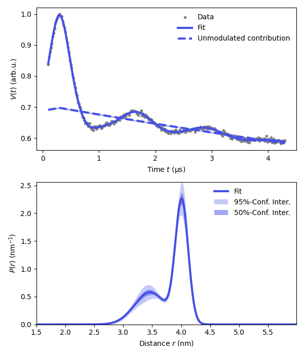
Basic analysis of a 4-pulse DEER signal with a bimodal Gaussian model

Fit a simple 4-pulse DEER signal with a model with a bimodal Gaussian parametric distribution and a homogeneous background.

import numpy as np
import matplotlib.pyplot as plt
import deerlab as dl

# File location
path = '../data/'
file = 'example_4pdeer_1.DTA'

# Experimental parameters
tau1 = 0.3      # First inter-pulse delay, μs
tau2 = 4.0      # Second inter-pulse delay, μs
tmin = 0.1      # Start time, μs

# Load the experimental data
t,Vexp = dl.deerload(path + file)

# Pre-processing
Vexp = dl.correctphase(Vexp) # Phase correction
Vexp = Vexp/np.max(Vexp)     # Rescaling (aesthetic)
t = t - t[0]                 # Account for zerotime
t = t + tmin

# Distance vector
r = np.arange(1.5,6,0.01) # nm

# Construct the model
Pmodel= dl.dd_gauss2
Vmodel = dl.dipolarmodel(t,r,Pmodel, experiment=dl.ex_4pdeer(tau1,tau2, pathways=[1]))

# Fit the model to the data
results = dl.fit(Vmodel,Vexp,reg=False)

# Print results summary
print(results)

Goodness-of-fit:
========= ============= ============= ===================== =======
 Dataset   Noise level   Reduced 𝛘2    Residual autocorr.    RMSD
========= ============= ============= ===================== =======
   #1         0.005         0.842             0.073          0.004
========= ============= ============= ===================== =======
Model parameters:
=========== ========= ========================= ====== =================================
 Parameter   Value     95%-Confidence interval   Unit   Description
=========== ========= ========================= ====== =================================
 mod         0.301     (0.299,0.303)                    Modulation depth
 reftime     0.300     (0.298,0.301)              μs    Refocusing time
 conc        149.186   (145.835,152.538)          μM    Spin concentration
 mean1       3.463     (3.400,3.526)              nm    1st Gaussian mean
 std1        0.269     (0.210,0.328)              nm    1st Gaussian standard deviation
 mean2       4.010     (4.000,4.020)              nm    2nd Gaussian mean
 std2        0.111     (0.099,0.123)              nm    2nd Gaussian standard deviation
 amp1        0.781     (0.756,0.806)                    1st Gaussian amplitude
 amp2        1.214     (1.190,1.238)                    2nd Gaussian amplitude
=========== ========= ========================= ====== =================================

# Extract fitted dipolar signal
Vfit = results.model

# Extract fitted distance distribution
Pfit = results.evaluate(Pmodel,r)
scale = np.trapz(Pfit,r)
Puncert = results.propagate(Pmodel,r,lb=np.zeros_like(r))
Pfit = Pfit/scale
Pci95 = Puncert.ci(95)/scale
Pci50 = Puncert.ci(50)/scale

# Extract the unmodulated contribution
Bfcn = lambda mod,conc,reftime: scale*(1-mod)*dl.bg_hom3d(t-reftime,conc,mod)
Bfit = results.evaluate(Bfcn)
Bci = results.propagate(Bfcn).ci(95)

plt.figure(figsize=[6,7])
violet = '#4550e6'
plt.subplot(211)
# Plot experimental and fitted data
plt.plot(t,Vexp,'.',color='grey',label='Data')
plt.plot(t,Vfit,linewidth=3,color=violet,label='Fit')
plt.plot(t,Bfit,'--',linewidth=3,color=violet,label='Unmodulated contribution')
plt.fill_between(t,Bci[:,0],Bci[:,1],color=violet,alpha=0.3)
plt.legend(frameon=False,loc='best')
plt.xlabel('Time $t$ (μs)')
plt.ylabel('$V(t)$ (arb.u.)')
# Plot the distance distribution
plt.subplot(212)
plt.plot(r,Pfit,color=violet,linewidth=3,label='Fit')
plt.fill_between(r,Pci95[:,0],Pci95[:,1],alpha=0.3,color=violet,label='95%-Conf. Inter.',linewidth=0)
plt.fill_between(r,Pci50[:,0],Pci50[:,1],alpha=0.5,color=violet,label='50%-Conf. Inter.',linewidth=0)
plt.legend(frameon=False,loc='best')
plt.autoscale(enable=True, axis='both', tight=True)
plt.xlabel('Distance $r$ (nm)')
plt.ylabel('$P(r)$ (nm$^{-1}$)')
plt.tight_layout()
plt.show()