Fitting Gaussians to a non-parametric distance distribution fit

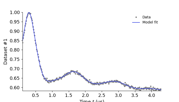
This example shows how to fit multi-Gaussian model to a non-parametric distance distribution calculated from Tikhonov regularization.

# Import the required libraries
import numpy as np
import matplotlib.pyplot as plt
import deerlab as dl

# File location
path = '../data/'
file = 'example_4pdeer_1.DTA'

# Experimental parameters
tau1 = 0.3      # First inter-pulse delay, μs
tau2 = 4.0      # Second inter-pulse delay, μs
tmin = 0.1      # Start time, μs

# Load the experimental data
t,Vexp = dl.deerload(path + file)

# Pre-processing
Vexp = dl.correctphase(Vexp) # Phase correction
Vexp = Vexp/np.max(Vexp)     # Rescaling (aesthetic)
t = t - t[0]                 # Account for zerotime
t = t + tmin

# Construct the dipolar signal model
r = np.arange(2,6,0.02)
Vmodel = dl.dipolarmodel(t,r, experiment = dl.ex_4pdeer(tau1,tau2, pathways=[1]))

# Fit the model to the data
results = dl.fit(Vmodel,Vexp)
results.plot(axis=t,xlabel='Time $t$ (μs)')
plt.show()

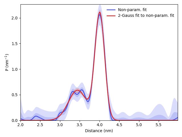
# From the fit results, extract the distribution
Pfit = results.P
Pci50 = results.PUncert.ci(50)
Pci95 = results.PUncert.ci(95)

# Select a bimodal Gaussian model for the distance distribution
Pmodel = dl.dd_gauss2
Pmodel.mean1.par0=3.5
Pmodel.mean2.par0=4.0

# Fit the Gaussian model to the non-parametric distance distribution
results = dl.fit(Pmodel,Pfit,r)

# Extract the fit results
PGauss = results.model
PGauss_uq = results.propagate(Pmodel,r,lb=np.zeros_like(r))
PGauss_ci50 = PGauss_uq.ci(50)
PGauss_ci95 = PGauss_uq.ci(95)

# Print the parameters nicely
print(f'Gaussian components with (95%-confidence intervals):')
print(f'       mean1 = {results.mean1:2.2f} ({results.mean1Uncert.ci(95)[0]:2.2f}-{results.mean1Uncert.ci(95)[1]:2.2f}) nm')
print(f'       mean2 = {results.mean2:2.2f} ({results.mean2Uncert.ci(95)[0]:2.2f}-{results.mean2Uncert.ci(95)[1]:2.2f}) nm')
print(f'        std1 = {results.std1:2.2f} ({results.std1Uncert.ci(95)[0]:2.2f}-{results.std1Uncert.ci(95)[1]:2.2f}) nm')
print(f'        std2 = {results.std2:2.2f} ({results.std2Uncert.ci(95)[0]:2.2f}-{results.std2Uncert.ci(95)[1]:2.2f}) nm')
print(f'  amplitude1 = {results.amp1:2.2f} ({results.amp1Uncert.ci(95)[0]:2.2f}-{results.amp1Uncert.ci(95)[1]:2.2f})')
print(f'  amplitude2 = {results.amp2:2.2f} ({results.amp2Uncert.ci(95)[0]:2.2f}-{results.amp2Uncert.ci(95)[1]:2.2f})')

Gaussian components with (95%-confidence intervals):
       mean1 = 3.44 (3.43-3.46) nm
       mean2 = 4.01 (4.00-4.01) nm
        std1 = 0.23 (0.22-0.25) nm
        std2 = 0.12 (0.12-0.13) nm
  amplitude1 = 0.69 (0.66-0.72)
  amplitude2 = 1.28 (1.27-1.30)

# Plot the fitted constraints model on top of the non-parametric case
violet = '#4550e6'
red = 'tab:red'
plt.plot(r,Pfit,linewidth=2,label='Non-param. fit',color=violet)
plt.fill_between(r,Pci50[:,0],Pci50[:,1],alpha=0.2,linewidth=0,color=violet)
plt.fill_between(r,Pci95[:,0],Pci95[:,1],alpha=0.2,linewidth=0,color=violet)
plt.plot(r,PGauss,linewidth=2,label='2-Gauss fit to non-param. fit',color=red)
plt.fill_between(r,PGauss_ci95[:,0],PGauss_ci95[:,1],alpha=0.2,linewidth=0,color=red)
# Formatting settings
plt.xlabel('Distance (nm)')
plt.ylabel('P (nm$^{-1}$)')
plt.autoscale(enable=True, axis='both', tight=True)
plt.legend(loc='best',frameon=False)
plt.tight_layout()
plt.show()