Fit a polynomial force field to a dipolar signal

This example shows how to extract a force fields (modelled as a polynomial function) from a dipolar signal.

# Import required libraries
import numpy as np
import matplotlib.pyplot as plt
import deerlab as dl

# Constants
R = 8.314            # universal gas constant, J/mol/K
T = 298              # Temperature for Boltzmann inversion (K)
kcal2J = 4.1868e3    # Conversion of kilocalories to J
thermal = R*T/kcal2J # Thermal energy in kcal/mol, (most force fields use this unit)

# Define the distance vector
r = np.linspace(2,6,300)

# Define the force field function (here modelled as a 3rd order polyomial)
def forcefield_energy(c0,c1,c2,c3):
    # Evaluate polynomial model for the force-field energy
    energy = np.polyval([c3,c2,c1,c0],r)
    # Shift to zero energy for the minimum
    energy += abs(energy.min())
    return energy

def forcefield_P(c0,c1,c2,c3):
    # Compute the energy
    energy = forcefield_energy(c0,c1,c2,c3)
    # Boltzmann distribution
    Pr = np.exp(-energy/thermal)
    # Ensure a probability density distribution
    Pr /= np.trapz(Pr,r)
    return Pr

# File location
path = '../data/'
file = 'example_4pdeer_4.DTA'

# Experimental parameters
tau1 = 0.3      # First inter-pulse delay, μs
tau2 = 5.0      # Second inter-pulse delay, μs
tmin = 0.1      # Start time, μs

# Load the experimental data
t,Vexp = dl.deerload(path + file)

# Pre-processing
Vexp = dl.correctphase(Vexp) # Phase correction
Vexp = Vexp/np.max(Vexp)     # Rescaling (aesthetic)
t = t - t[0]                     # Account for zerotime
t = t + tmin

# Construct the energy and distance distribution models
forcefield_energymodel = dl.Model(forcefield_energy)
forcefield_Pmodel = dl.Model(forcefield_P)

# Set boundaries and initial conditions
forcefield_Pmodel.c1.set(lb=-4,  ub=1, par0=0)
forcefield_Pmodel.c2.set(lb=-4,  ub=1, par0=0)
forcefield_Pmodel.c3.set(lb=-4,  ub=1, par0=0)
forcefield_Pmodel.c0.set(lb=-4,  ub=1, par0=0)

# Construct the dipolar signal model
Vmodel = dl.dipolarmodel(t,r,Pmodel=forcefield_Pmodel,Bmodel=dl.bg_hom3d,experiment=dl.ex_4pdeer(tau1,tau2,pathways=[1]))

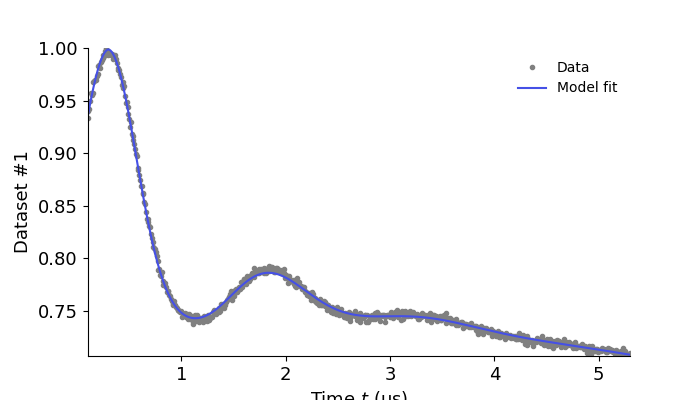
# Fit the model to the data
results = dl.fit(Vmodel,Vexp)

results.plot(axis=t, xlabel='Time $t$ (μs)')
plt.show()

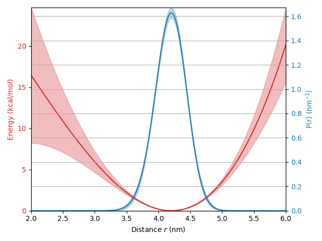
# Evaluate the models at the fitted parameters
Pfit = forcefield_Pmodel(results.c0,results.c1,results.c2,results.c3)
energy = forcefield_energymodel(results.c0,results.c1,results.c2,results.c3)

# Propagate the fit uncertainty to the models
Puq = results.propagate(forcefield_Pmodel, lb=np.zeros_like(r))
energyuq = results.propagate(forcefield_energymodel, lb=np.zeros_like(r))

# Plot the results
fig, ax1 = plt.subplots()

color = 'tab:red'
ax1.plot(r, energy, color=color)
ax1.fill_between(r,energyuq.ci(95)[:,0],energyuq.ci(95)[:,1],alpha=0.3,color=color)
ax1.tick_params(axis='y', labelcolor=color)
ax1.set_ylabel('Energy (kcal/mol)', color=color)  # we already handled the x-label with ax1
ax1.set_xlabel('Distance $r$ (nm)')

ax2 = ax1.twinx()  # instantiate a second axes that shares the same x-axis

color = 'tab:blue'
ax2.plot(r, Pfit, color=color)
ax2.fill_between(r,Puq.ci(95)[:,0],Puq.ci(95)[:,1],alpha=0.3,color=color)
ax2.tick_params(axis='y', labelcolor=color)
ax2.set_ylabel('P(r) (nm$^{-1}$)', color=color)
ax2.grid(None)

ax1.autoscale(enable=True, axis='both', tight=True)
ax2.autoscale(enable=True, axis='both', tight=True)
fig.tight_layout()  # otherwise the right y-label is slightly clipped
plt.show()