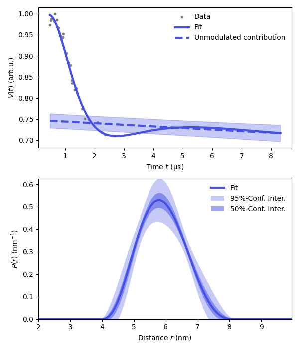
Basic analysis of a sparsely sampled 4-pulse DEER signal

Fit a simple sparsely 4-pulse DEER signal (only 10% of the points have been sampled) with a model with a non-parametric distribution and a homogeneous background, using Tikhonov regularization.

Nota that no modifications are required when analyzing sparse sampled data in contrast to densely sampled data.

import numpy as np
import matplotlib.pyplot as plt
import deerlab as dl

# File location
path = '../data/'
datafile = 'experimental_sparse_ptbp1_4pdeer.DTA'
timingsfile = 'experimental_sparse_4pdeer_timings.DTA'

# Experimental parameters
tau1 = 0.400      # First inter-pulse delay, μs
tau2 = 8.000      # Second inter-pulse delay, μs
tmin = 0.482      # Start time, μs

# Load the experimental data and the grid of recorded timings (this depends on how the data were acquired)
_,Vexp = dl.deerload(path + datafile)
_,t = dl.deerload(path + timingsfile)
t = t/1000 # ns -> μs

# Pre-processing
Vexp = dl.correctphase(Vexp) # Phase correction
Vexp = Vexp/np.max(Vexp)     # Rescaling (aesthetic)
t = t - t[0]                     # Account for zerotime
t = t + tmin

# Distance vector
r = np.arange(2,10,0.05) # nm

# Construct the model with the sparse sampled time vector
Vmodel = dl.dipolarmodel(t,r, experiment = dl.ex_4pdeer(tau1,tau2, pathways=[1]))
compactness = dl.dipolarpenalty(Pmodel=None, r=r, type='compactness')

# Fit the model to the data
results = dl.fit(Vmodel,Vexp, penalties = compactness)

# Print results summary
print(results)

Goodness-of-fit:
========= ============= ============= ===================== =======
 Dataset   Noise level   Reduced 𝛘2    Residual autocorr.    RMSD
========= ============= ============= ===================== =======
   #1         0.012         0.818             0.845          0.011
========= ============= ============= ===================== =======
Model hyperparameters:
========================== ===================
 Regularization parameter   Penalty weight #1
========================== ===================
          1.859                 6.50e-04
========================== ===================
Model parameters:
=========== ======== ========================= ====== ======================================
 Parameter   Value    95%-Confidence interval   Unit   Description
=========== ======== ========================= ====== ======================================
 mod         0.252    (0.235,0.268)                    Modulation depth
 reftime     0.444    (0.352,0.448)              μs    Refocusing time
 conc        20.617   (12.342,28.891)            μM    Spin concentration
 P           ...      (...,...)                 nm⁻¹   Non-parametric distance distribution
 P_scale     0.998    (0.987,1.008)             None   Normalization factor of P
=========== ======== ========================= ====== ======================================

# Evaluate the fitted dipolar signal over the densely sampled vector
dt = min(np.diff(t))
tuniform = np.arange(min(t),max(t),dt)
Vuniform = dl.dipolarmodel(tuniform,r, experiment = dl.ex_4pdeer(tau1,tau2, pathways=[1]))
Vfit = results.evaluate(Vuniform)

# Extract fitted distance distribution
Pfit = results.P
Pci95 = results.PUncert.ci(95)
Pci50 = results.PUncert.ci(50)

# Extract the unmodulated contribution
Bfcn = lambda mod,conc,reftime: results.P_scale*(1-mod)*dl.bg_hom3d(tuniform-reftime,conc,mod)
Bfit = results.evaluate(Bfcn)
Bci = results.propagate(Bfcn).ci(95)

plt.figure(figsize=[6,7])
violet = '#4550e6'
plt.subplot(211)
# Plot experimental and fitted data
plt.plot(t,Vexp,'.',color='grey',label='Data')
plt.plot(tuniform,Vfit,linewidth=3,color=violet,label='Fit')
plt.plot(tuniform,Bfit,'--',linewidth=3,color=violet,label='Unmodulated contribution')
plt.fill_between(tuniform,Bci[:,0],Bci[:,1],color=violet,alpha=0.3)
plt.legend(frameon=False,loc='best')
plt.xlabel('Time $t$ (μs)')
plt.ylabel('$V(t)$ (arb.u.)')
# Plot the distance distribution
plt.subplot(212)
plt.plot(r,Pfit,color=violet,linewidth=3,label='Fit')
plt.fill_between(r,Pci95[:,0],Pci95[:,1],alpha=0.3,color=violet,label='95%-Conf. Inter.',linewidth=0)
plt.fill_between(r,Pci50[:,0],Pci50[:,1],alpha=0.5,color=violet,label='50%-Conf. Inter.',linewidth=0)
plt.legend(frameon=False,loc='best')
plt.autoscale(enable=True, axis='both', tight=True)
plt.xlabel('Distance $r$ (nm)')
plt.ylabel('$P(r)$ (nm$^{-1}$)')
plt.tight_layout()
plt.show()