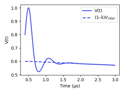
Simulating a 4-pulse DEER signal

An example on how to simulate a basic 4-pulse DEER dipolar signal, with the main dipolar pathway (i.e. without other contributions such as 2+1). This example uses a Gaussian distance distribution.

# Import the required libraries
import numpy as np
import matplotlib.pyplot as plt
import deerlab as dl

# Simulation parameters
tau1, tau2 = 0.5, 2.5 # Inter-pulse delays, µs
tmin = 0.4            # Start time, μs
Δt = 0.008            # Time increment, μs

rmean = 3.0           # Mean distance, nm
rstd = 0.2            # Distance standard deviation, nm
rmin, rmax = 1.5, 6   # Range of the distance vector, nm
Δr = 0.05             # Distance increment, nm

conc = 50             # Spin concentration, μM
lam = 0.40            # Modulation depth
V0 = 1                # Overall echo amplitude

# Time vector
tmax = tau1+tau2
t = np.arange(tmin, tmax, Δt)

# Distance vector
r = np.arange(rmin, rmax, Δr)

# Construct the 4-pulse DEER model
Vmodel = dl.dipolarmodel(t, r, Pmodel=dl.dd_gauss)

# Simulate the signal with orientation selection
Vsim = Vmodel(mean=rmean, std=rstd, conc=conc, scale=V0, mod=lam, reftime=tau1)

# Scaled background (for plotting)
Vinter = V0*(1-lam)*dl.bg_hom3d(t-tau1, conc, lam)

# Plot the simulated signal
violet = '#4550e6'
plt.figure(figsize=[4,3])
plt.plot(t, Vsim, color=violet, lw=2, label='V(t)')
plt.plot(t, Vinter, '--', color=violet, lw=2, label='(1-λ)$V_{inter}$')
plt.legend()
plt.xlabel('Time (μs)')
plt.ylabel('V(t)')
plt.tight_layout()
plt.show()